Download
1 / 12
120 likes | 252 Views
Analysis of Hyperspectral Image Using Minimum Volume Transform (MVT). Ziv Waxman & Chen Vanunu Instructor: Mr. Oleg Kuybeda. Objectives:. Testing the MVT algorithm as a tool of analyzing hyperspectral image.

E N D
Analysis of Hyperspectral Image Using Minimum Volume Transform (MVT) Ziv Waxman & Chen Vanunu Instructor: Mr. Oleg Kuybeda
Objectives: • Testing the MVT algorithm as a tool of analyzing hyperspectral image. • Obtain end-members (pure spectral signatures) present in hyperspectral image as output.
Analysis Steps • Pre-processing: rank and end-members estimation (MOCA algorithm). • Data Depletion (select data upon convex hull). • Run MVT (apply linear programming) and concurrently perform constraints depletion. • Get end-members and compare with MOCA end-members. MOCA end-members Pre-processing Data depletion MVT compare MVT end-members
Assumptions • LMM – Linear Mixture Model. Every pixel is a linear combination of pure spectral signatures (end members). • End members are linearly independent. • Pixels-scatter-diagram is convex. Located in the first octant (for 3D).
MVT Variants • Dark Point Fixed (DPFT) - dark point reliably known. - better when no bias. • Fixed Point Free (FPFT) - dark point not known. - better when constant bias applied to data.
Pixels-Scatter-Diagram for 3-Bands Dist. • Generally looks like a “tear drop”. • Pi represent the end members. Define facets of a minimum volume circumscribing simplex. P2 This facet is x+y+z=1 P1 dark point data P3 O
MVT Algorithm – DPFT DFPT selected – due to random bias applied by scanner. Create simplex without moving actual data. Project data onto uTx=1 Data Depletion Create start simplex k=1 Rotate k’th facet (linear programming – simplex method) Get constraints and deplete them End members k=k+1 If k=n+1 then k=1
Data Depletion • Only data points upon the convex hull define a simplex. • Choose these points by applying variant of Gram-Schmidt orthogonalization process. • should leave 10% of total data.
Constraints Depletion • Applied when data depletion process leaves too many points. • Remove redundant constraints, which do not contribute to creation of feasible region (linear programming). Feasible region Feasible region
Synthetic data results • Blue circled – MOCA end-members • Red points – after data depletion • Azure – MVT end-members Arial view: - White noise applied - Constant bias applied
Real image results • random bias • Three images represent each end member
Discussion • Creates a minimum volume simplex for a given data. • Extremely efficient when bias is constant. • Preserves rare-vectors – MOCA and MVT do not ignore abnormalities in an image. • MVT is very sensitive to random bias. • Sensitive to noise.