Download
1 / 21
260 likes | 507 Views
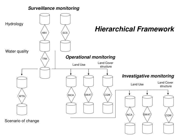
HBV. SCS. TRK. WTN. SWAT. SWAT. CQW. CQW. INCA. INCA. Surveillance monitoring. Hydrology. Hierarchical Framework. Water quality. Operational monitoring. Land Cover structure. Land Use. Investigative monitoring. Land Cover structure. Land Use. Scenario of change.

E N D
HBV SCS TRK WTN SWAT SWAT CQW CQW INCA INCA Surveillance monitoring Hydrology Hierarchical Framework Water quality Operational monitoring Land Cover structure Land Use Investigative monitoring Land Cover structure Land Use Scenario of change
Data requirement for HBV Input data are observations of precipitation, air temperature and estimates of potential evapotranspiration. The time step is usually one day, but it is possible to use shorter time steps. The evaporation values used are normally monthly averages although it is possible to use daily values. Air temperature data are used for calculations of snow accumulation and melt. It can also be used to adjust potential evaporation when the temperature deviates from normal values, or to calculate potential evaporation. If none of these last options are used, temperature can be omitted in snow free areas.
Information on HBV model The HBV model (Bergström, 1976, 1992) is a rainfall-runoff model, which includes conceptual numerical descriptions of hydrological processes at the catchment scale. The general water balance can be described as: where: P = precipitation E = evapotranspiration Q = runoff SP = snow pack SM = soil moisture UZ = upper groundwater zone LZ =lower groundwater zone lakes = lake volume The standard snowmelt routine of the HBV model is a degree-day approach, based on air temperature, with a water holding capacity of snow which delays runoff. Melt is further distributed according to the temperature lapse rate and is modeled differently in forests and open areas. A threshold temperature, TT, is used to distinguish rainfall from snowfall. Although the automatic calibration routine is not a part of the model itself, it is an essential component in the practical work. The standard criterion (Lindström, b1997) is a compromise between the traditional efficiency, R2 by Nash and Sutcliffe (1970) and the relative volume error, RD: In practice the optimisation of only R2 often results in a remaining volume error. The criterion above gives results with almost as high R2 values and practically no volume error. The best results are obtained with w close to 0.1. The automatic calibration method for the HBV model developed by Harlin (1991) used different criteria for different parameters. With the simplification to one single criterion, the search method could be made more efficient. The optimisation is made for one parameter at a time, while keeping the others constant. The one-dimensional search is based on a modification of the Brent parabolic interpolation (Press et al., 1992). Description of the HBV model captured from: http://www.smhi.se/sgn0106/if/hydrologi/hbv.htm Link to official homepage: http://www.smhi.se/foretag/m/hbv_demo/html/welcome.html
Information on HBV output In different model versions HBV has been applied in more than 40 countries all over the world. The model is used for flood forecasting in the Nordic countries, and many other purposes, such as spillway design floods simulation (Bergström et al., 1992), water resources evaluation (for example Jutman, 1992, Brandt et al., 1994), nutrient load estimates (Arheimer, 1998). It is possible to run the model separately for several sub basins and then add the contributions from all sub basins. Calibration as well as forecasts can be made for each sub basin. For basins of considerable elevation range a subdivision into elevation zones can also be made.
Information on SCS data requirement The data requirements for this method are very low, rainfall amount and curve number. The curve number is based on the area's hydrologic soil group, land use, treatment and hydrologic condition. The last two variables are of greatest importance.
precipitation surface Evapo- runoff transpiration Root zone Unsaturated Zone Saturated Zone Deep Aquifer infiltration percolation deep loss Information on SCS model The general equation for the SCS curve number method is as follows: The initial equation (1) is based on trends observed in data from collected sites; therefore it is an empirical equation instead of a physically based equation. After further empirical evaluation of the trends in the data base, the initial abstractions, Ia, could be defined as a percentage of S (2). With this assumption, the equation (3) could be written in a more simplified form with only 3 variables. The parameter CN is a transformation of S, and it is used to make interpolating, averaging, and weighting operations more linear (4). Curve numbers are available for most land-use types. lateral flow return flow ( Slide from W. Bauwens, 2006 ) Description of the SCS method captured from: http://www.ecn.purdue.edu/runoff/documentation/scs.htm
Information on SCS model output The SCS curve number method is a simple, widely used and efficient method for determining the amount of runoff from a rainfall even in a particular area. The SCS curve number method is often included in more advanced hydrological models to evaluate surface runoff (e.g. HBV and SWAT). Although the method is designed for a single storm event, it can be scaled to find average annual runoff values.
Information on TRK model The TRK system combines: 1. Preparation of areal distribution of different land-use categories and positioning of point sources using GIS; 2. Calculations of concentration and area losses of diffuse sources (for N from arable land by using the dynamic soil profile model SOILNDB); 3. Calculations of the water balance (by using the distributed dynamic HBV model) and N transport and retention processes in water (by using the model HBV-N).
Information on TRK model output The results are presented in the GIS, and source apportionment is made for each sub-basin as well as for the whole river basins. The results from the system have been used for international reports on the transport to the sea, for assessment of the reduction of the anthropogenic load on the sea and for guidance on effective measures for reducing the load on the sea on a national scale.
Data input for WATSHMAN Map themes • Basic maps • Sub catchments • Streams • Lakes • Elevation data • Soil maps • Land use Tabular information • Point sources • Climate data • Monitoring data • Model results Main input form
Data output from WATSHMAN - Data management and presentation options such as selecting, editing, simple calculations and usual GIS functions. - Nutrient transport options with chains of models such as diffuse leakage, lake retention model etc. - Scenario management options such as changes in crop, landuse, sewage treatment etc.
Information on INCA model Instream processes Land component A.J. Wade, P. Durand, V. Beaujouan, W.W. Wessel, K.J. Raat, P.G. Whitehead, D. Butterfield, K. Rankinen and A. Lepisto (2002), A nitrogen model for European catchments: INCA, new model structure and equations. Hydrol.Earth Syst. Sci., 6(3) 559-582.
Output data from INCA model Land component output Instream component output
Data input for SWAT model Soil Map. For each soil layer: Textural properties: Physico-chemical-properties: Landuse Map Landuse information: crop, water bodies (lake,pond, etc.) Cropping information: planting and harvest date, yield, etc. Management practices: fertilizer and pesticide application timing and amount Climate Information Daily rainfall, minimum and maximum air temperature, net solar radiation Monthly average wind speed Average monthly humidity Water Quality Information Point sources Location Average daily flow Average daily sediment and nutrient loading Hydrogeological Map Groundwater abstraction timing and amount Digital Elevation Model Monitoring Data for model calibration: Observed flows at subbasin /basin outlet(s) Nutrient loadings at subbasin/basin outlet (s) Sediment loadings at subbasin/basin outlet(s) Main validation data required Observed flows at subbasin /basin outlet(s) Nutrient loadings at subbasin/basin outlet (s) Sediment loadings at subbasin/basin outlet(s)
Information on SWAT model SWAT uses a two-level dissagregation scheme; a preliminary subbasin identification is carried out based on topographic criteria, followed by further discretization using land use and soil type considerations. The physical properties inside each subbasin are then aggregated with no spatial significance. The time step for the simulation can be daily, monthly or yearly, which qualify the model for long-term simulations. Reference Model description : Neitsch S.L., Arnold J.G., Kiniry J.R., Williams J.R., (2001), Soil and Water Assessment Tool – Theoretical Documentation - Version 2000, Blackland Research Center – Agricultural Research Service, Texas – USA Reference Users guide: Neitsch S.L., Arnold J.G., Kiniry J.R., Williams J.R., (2001), Soil and Water Assessment Tool – User Manual Version 2000, Blackland Research Center Agricultural Research Service, Texas – USA
Data output from SWAT It predicts the long-term impacts in large basins of management and also timing of agricultural practices within a year (i.e., crop rotations, planting and harvest dates, irrigation, fertilizer, and pesticide application rates and timing). It can be used to simulate at the basin scale water and nutrients cycle in landscapes whose dominant land use is agriculture It can also help in assessing the environmental efficiency of BMP’s and alternative management policies.
Data input for CEQUALW2 model The model has been widely applied to stratified surface water systems such as lakes, reservoirs, and estuaries and computes water levels, horizontal and vertical velocities, temperature, and 21 other water quality parameters (such as dissolved oxygen, nutrients, organic matter, algae, pH, the carbonate cycle, bacteria, and dissolved and suspended solids). Version 3 has the capability of modeling entire river basins with rivers and inter-connected lakes, reservoirs, and/or estuaries.
information on CEQUALW2 model A predominant feature of the model is its ability to compute the two-dimensional velocity field for narrow systems that stratify. In contrast with many reservoir models that are zero-dimensional with regards to hydrodynamics, the ability to accurately simulate transport can be as important as the water column kinetics in accurately simulating water quality. Link to CE-QUAL-W2 homepagehttp://www.ce.pdx.edu/w2/
Data output from CEQUALW2 model CE-QUAL-W2 has been in use for the last two decades as a tool for water quality managers to assess the impacts of management strategies on reservoir, lake, and estuarine systems. CE-QUAL-W2 is a two-dimensional water quality and hydrodynamic code supported by the USACE Waterways Experiments Station (Cole and Buchak). W2 models basic eutrophication processes such as temperature-nutrient-algae-dissolved oxygen-organic matter and sediment relationships.