Introduction

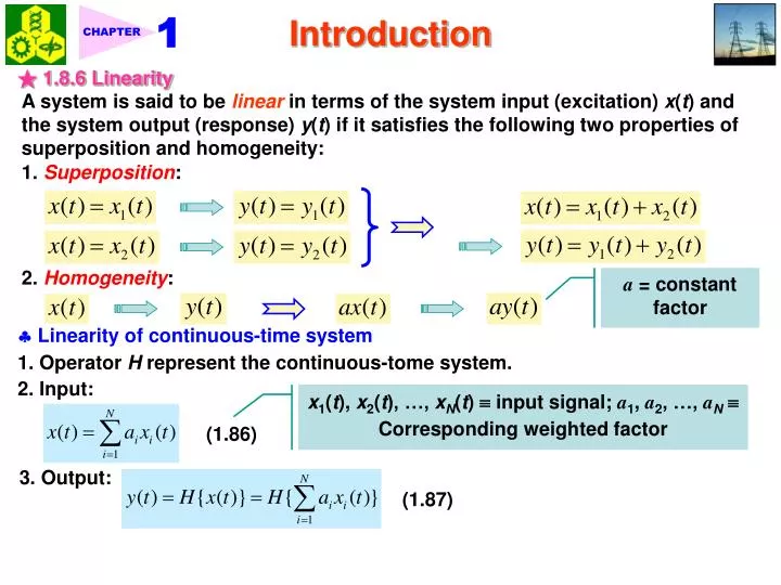
1. 1 CHAPTER Introduction ★ 1.8.6 Linearity A system is said to be linear in terms of the system input (excitation) x(t) and the system output (response) y(t) if it satisfies the following two properties of superposition and homogeneity: 1. Superposition: 2. Homogeneity: a = constant factor  Linearity of continuous-time system 1. Operator H represent the continuous-tome system. 2. Input: x1(t), x2(t), …, xN(t)  input signal; a1, a2, …, aN  Corresponding weighted factor (1.86) 3. Output: (1.87)

2. 1 CHAPTER Introduction Superposition and homogeneity (1.88) where (1.89) 4. Commutation and Linearity: (1.90) Fig. 1.56  Linearity of discrete-time system Same results, see Example 1.19. Example 1.19 Linear Discrete-Time system Consider a discrete-time system described by the input-output relation Show that this system is linear.

3. 1 CHAPTER Introduction Figure 1.56 (p. 64)The linearity property of a system. (a) The combined operation of amplitude scaling and summation precedes the operator H for multiple inputs. (b) The operator H precedes amplitude scaling for each input; the resulting outputs are summed to produce the overall output y(t). If these two configurations produce the same output y(t), the operator H is linear. <p.f.> 1. Input: 2. Resulting output signal:

4. 1 CHAPTER Introduction where Linear system! Example 1.20 Nonlinear Continuous-Time System Consider a continuous-time system described by the input-output relation Show that this system is nonlinear. <p.f.> 1. Input: 2. Output: Here we cannot write Nonlinear system!

5. 1 CHAPTER 1/ /2 /2 Introduction Example 1.21 Impulse Response of RC Circuit For the RC circuit shown in Fig. 1.57, determine the impulse response y(t). <Sol.> 1. Recall: Unit step response Figure 1.57 (p. 66)RC circuit for Example 1.20, in which we are given the capacitor voltage y(t) in response to the step input x(t) = y(t) and the requirement is to find y(t) in response to the unit-impulse input x(t) = (t). (1.91) 2. Rectangular pulse input: Fig. 1.58. x(t) = x(t) Figure 1.58 (p. 66)Rectangular pulse of unit area, which, in the limit, approaches a unit impulse as Δ0. 3. Response to the step functions x1(t) and x2(t):

6. 1 CHAPTER Introduction Next, recognizing that i) (t) = the limiting form of the pulse x(t): (1.92)

7. 1 CHAPTER Introduction ii) The derivative of a continuous function of time, say, z(t): (1.92) Cancel each other! (1.93)

8. 1 CHAPTER Introduction 1.9 Noise Noise  Unwanted signals 1. External sources of noise: atmospheric noise, galactic noise, and human- made noise. 2. Internal sources of noise: spontaneous fluctuations of the current or voltage signal in electrical circuit. (electrical noise) Fig. 1.60. ★ 1.9.1 Thermal Noise Thermal noise arises from the random motion of electrons in a conductor. Two characteristics of thermal noise: 1. Time-averaged value: 2T = total observation interval of noise (1.94) As T  , Refer to Fig. 1.60. 2. Time-average-squared value: k = Boltzmann’s constant = 1.38  10 23 J/K Tabs = absolute temperature (1.95) As T , (1.96)

9. 1 CHAPTER Introduction Figure 1.60 (p. 68)Sample waveform of electrical noise generated by a thermionic diode with a heated cathode. Note that the time-averaged value of the noise voltage displayed is approximately zero.

10. 1 CHAPTER Introduction  Thevenin’s equvalent circuit: Fig. 1.61(a), Norton’s equivalent circuit: Fig. 1.61(b). Noise voltage generator: Noise current generator: (1.97) where G = 1/R = conductance [S].  Maximum power transfer theorem: the maximum possible power is transferred from a source of internal resistance R to a load of resistance RlwhenR = Rl. Figure 1.61 (p. 70)(a) Thévenin equivalent circuit of a noisy resistor. (b) Norton equivalent circuit of the same resistor. Under matched condition, the available power is

11. 1 CHAPTER Introduction  Two operating factor that affect available noise power: 1. The temperature at which the resistor is maintained. 2. The width of the frequency band over which the noise voltage across the resistor is measured. ★ 1.9.2 Other Sources of Electrical Noise 1. Shot noise: the discrete nature of current flow electronic devices 2. Ex. Photodetector: 1) Electrons are emitted at random times, k, where  < k <  2) Total current flowing through photodetector: (1.98) is the current pulse generated at time k. where 3. 1/f noise: The electrical noise whose time-averaged power at a given frequency is inversely proportional to the frequency.

12. 1 CHAPTER x(t) y(t) differentiator Introduction 1.10 Theme Example ★ 1.10.1 Differentiation and Integration: RC Circuits 1. Differentiator  Sharpening of a pulse (1.99) 1) Simple RC circuit: Fig. 1.62. 2) Input-output relation: (1.100) Figure 1.62 (p. 71)Simple RC circuit with small time constant, used as an approximator to a differentiator. If RC (time constant) is small enough such that (1.100) is dominated by the second term v2(t)/RC, then (1.101)

13. 1 CHAPTER x(t) y(t) integrator Introduction Input: x(t) = RCv1(t); output: y(t) = v2(t) 2. Integrator  smoothing of an input signal (1.102) 1) Simple RC circuit: Fig. 1.63. 2) Input-output relation: (1.103) If RC (time constant) is large enough such that (1.103) is dominated by the first term RCv2(t), then Figure 1.63 (p. 72)Simple RC circuit with large time constant used as an approximator to an integrator. Input: x(t) = [1/(RC)v1(t)];output: y(t) = v2(t)

14. 1 CHAPTER Introduction ★ 1.10.2 MEMS Accelerometer 1. Model: second-order mass-damper-spring system Fig. 1.64. M = proof mass, K = effective spring constant, D = damping factor, x(t) =external acceleration, y(t) =displacement of proof mass, Md2y(t)/dt2 = inertial force of proof mass, Ddy(t)/dt = damping force, Ky(t) = spring force. 2. Force Eq.: Figure 1.64 (p. 73)Mechanical lumped model of an accelerometer. (1.105) 1) Natural frequency: 2) Quality factor: [rad/sec] (1.106) (1.107)

15. 1 CHAPTER Introduction (1.105) (1.108) ★ 1.10.3 Radar Range Measurement 1. A periodic sequence of radio frequency (RF) pulse: Fig. 1.65. T0 = duration [sec], 1/T = repeated frequency, fc = RF frequency [MHz~GHz] Figure 1.65 (p. 74)Periodic train of rectangular FR pulses used for measuring molar ranges.  The sinusoidal signal acts as a carrier.

16. 1 CHAPTER Introduction 2. Round-trip time = the time taken by a radar pulse to reach the target and for the echo from the target to come back to the radar. (1.109) d = radar target range, c = light speed. 3. Two issues of concern in range measurement: 1) Range resolution: The duration T0 of the pulse places a lower limit on the shortest round-trip delay time that the radar can measure. Smallest target range: dmin = cT0/2 [m] 2) Range ambiguity: The interpulse period T places an upper limit on the largest range that the radar can measure. Largest target range: dmax = cT/2 [m] ★ 1.10.4 Moving-Average Systems 1. N-point moving-average system: Fig. 1.66. (1.110) x(t) = input signal The value N determines the degree to which the system smooths the input data.

17. 1 CHAPTER Introduction Figure 1.66a (p. 75)(a) Fluctuations in the closing stock price of Intel over a three-year period.

18. 1 CHAPTER Introduction Figure 1.66b (p. 76)(b) Output of a four-point moving-average system. N = 4 case

19. 1 CHAPTER Introduction Figure 1.66c (p. 76)(c) Output of an eight-point moving-average system. N = 8 case

20. 1 CHAPTER Introduction 2. For a general moving-average system, unequal weighting is applied to past values of the input: (1.111) ★ 1.10.5 Multipath Communication Channels 1. Channel noise degrades the performance of a communication system. 2. Another source of degradation of channel: dispersive nature, i.e., the channel has memory. 3. For wireless system, the dispersive characteristics result from multipath propagation. Fig. 1.67.  For a digital communication, multipath propagation manifests itself in the form of intersymbol interference (ISI). 4. Baseband model for multipath propagation: Tapped-delay line  Fig. 1.68. Tdiff = smallest time difference between different path (1.112)

21. 1 CHAPTER Introduction Figure 1.67 (p. 77)Example of multiple propagation paths in a wireless communication environment.

22. 1 CHAPTER Introduction Figure 1.68 (p. 78)Tapped-delay-line model of a linear communication channel, assumed to be time-invariant.

23. 1 CHAPTER Introduction 5. PTdiff = the longest time delay of any significant path relative to the arrival of the signal. The coefficients wi are used to approximate the gain of each path. For P =1, then 0x(t) = direct path, 1x(tTdiff) = single reflected path 6. Discrete-time case: Linearly weighted moving-average system (1.113) The term recursive signifies the dependence of the output signal on its own past values. For P =1, then (1.114) ★ 1.10.6 Recursive Discrete-Time Computations 1. First-order recursive discrete-time filter: Fig. 1.69. (1.115) x[n] = input, y[n] = output where  is a constant.

24. 1 CHAPTER Introduction Figure 1.69 (p. 79)Block diagram of first-order recursive discrete-time filter. The operator S shifts the output signal y[n] by one sampling interval, producing y[n – 1]. The feedback coefficient  determines the stability of the filter.  Fig. 1.69: linear discrete-time feedback system. 2. Solution of Eq.(1.115): r   (1.116) (1.117) Setting k 1 = l, Eq.(1.117) becomes (1.118)

25. 1 CHAPTER Introduction 3. Three special cases (depending on ): Accumulator 1)  = 1: (1.116) (1.119) 2) Leaky accumulator Stable in BIBO sense 3) Amplified accumulator Unsatble in BIBO sense 1.11 Exploring Concepts with MATLAB  MATLAB Signal Processing Toolbox 1. Time vector: Sampling interval Ts of 1 ms on the interval from 0 to 1 s t = 0:.001:1; 2. Vector n: n = 0:1000; ★ 1.11.1 Periodic Signals 1. Square wave: A =amplitude, w0 = fundamental frequency, rho = duty cycle A*square(w0*t, rho);

26. 1 CHAPTER Introduction Ex. Obtain the square wave shown in Fig. 1.14 (a) by using MATLAB. <Sol.> >> A = 1; >> w0 =10*pi; >> rho = 0.5; >> t = 0:.001:1; >> sq = A*square(w0*t, rho); >> plot (t, sq) >> axis([0 1 -1.1 1.1]) 2. Triangular wave: A =amplitude, w0 = fundamental frequency, w = width A*sawtooth(w0*t, w); Ex. Obtain the triangular wave shown in Fig. 1.15 by using MATLAB. <Sol.> >> A = 1; >> w0 =10*pi; >> w = 0.5; >> t = 0:0.001:1; >> tri = A*sawtooth(w0*t, w); >> plot (t, tri)

27. 1 CHAPTER Introduction 3. Discrete-time signal: stem(n, x); x = vector, n = discrete time vector Ex. Obtain the discrete-time square wave shown in Fig. 1.16 by using MATLAB. <Sol.> >> A = 1; >> omega =pi/4; >> n = -10:10; >> x = A*square(omega*n); >> stem(n, x) 4. Decaying exponential: B*exp(-a*t); Growing exponential: B*exp(a*t); Ex. Obtain the decaying exponential signal shown in Fig. 1.28 (a) by using MATLAB. <Sol.> >> B = 5; >> a = 6; >> t = 0:.001:1; >> x = B*exp(-a*t); % decaying exponential >> plot (t, x)

28. 1 CHAPTER Introduction Ex. Obtain the growing exponential signal shown in Fig. 1.28 (b) by using MATLAB. <Sol.> >> B = 1; >> a = 5; >> t = 0:0.001:1; >> x = B*exp(a*t); % growing exponential >> plot (t, x) Ex. Obtain the decaying exponential sequence shown in Fig. 1.30 (a) by using MATLAB. <Sol.> >> B = 1; >> r = 0.85; >> n = -10:10; >> x = B*r.^n; % decaying exponential sequence >> stem (n, x) A = amplitude, w0 = frequency, phi = phase angle ★ 1.11.3 Sinusoidal Signals 1. Cosine signal: 2. Sine signal: A*cos(w0*t + phi); A*sin(w0*t + phi);

29. 1 CHAPTER Introduction Ex. Obtain the sinusoidal signal shown in Fig. 1.31 (a) by using MATLAB. <Sol.> >> A = 4; >> w0 =20*pi; >> phi = pi/6; >> t = 0:.001:1; >> cosine = A*cos(w0*t + phi); >> plot (t, cosine) Ex. Obtain the discrete-time sinusoidal signal shown in Fig. 1.33 by using MATLAB. <Sol.> >> A = 1; >> omega =2*pi/12; % angular frequency >> n = -10:10; >> y = A*cos(omega*n); >> stem (n, y) .* element-by-element multiplication ★ 1.11.4 Exponential Damped Sinusoidal Signals 1. Exponentially damped sinusoidal signal: MATLAB Format: A*sin(w0*t + phi).*exp(-a*t);

30. 1 CHAPTER Introduction Ex. Obtain the waveform shown in Fig. 1.35 by using MATLAB. <Sol.> >> A = 60; >> w0 =20*pi; >> phi = 0; >> a = 6; >> t = 0:.001:1; >> expsin = A*sin(w0*t + phi).*exp(-a*t); >> plot (t, expsin) Ex. Obtain the exponentially damped sinusoidal sequence shown in Fig. 1.70 by using MATLAB. <Sol.> >> A = 1; >> omega =2*pi/12; % angular frequency >> n = -10:10; >> y = A*cos(omega*n); >> r = 0.85; >> x = A*r.^n; % decaying exponential sequence >> z = x.*y; % elementwise multiplication >> stem (n, z)

31. 1 CHAPTER Introduction Figure 1.70 (p. 84)Exponentially damped sinusoidal sequence.

32. 1 CHAPTER Introduction ★ 1.11.5 Step, Impulse, and Ramp Functions Ex. Generate a rectangular pulse centered at origin on the interval [-1, 1]. ◆ MATLAB command: 1. M-by-N matrix of ones: ones (M, N) 2. M-by-N matrix of zeros: zeros (M, N) <Sol.>  Unit amplitude step function: >> t = -1:1/500:1; >> u1 = [zeros(1, 250), ones(1, 751)]; >> u2 = [zeros(1, 751), ones(1, 250)]; >> u = u1 – u2; u = [zeros(1, 50), ones(1, 50)];  Discrete-time impulse: delta = [zeros(1, 49), 1, zeros(1, 49)];  Ramp sequence: ramp = 0:.1:10 ★ 1.11.6 User-Defined Functions 1. Two types M-files exist: scripts and functions. Scripts, or script files automate long sequences of commands; functions, or function files, provide extensibility to MATLAB by allowing us to add new functions. 2. Procedure for establishing a function M-file:

33. 1 CHAPTER Introduction 1) It begins with a statement defining the function name, its input arguments, and its output arguments. 2) It also includes additional statements that compute the values to be returned. 3) The inputs may be scalars, vectors, or matrices. Ex. Obtain the rectangular pulse depicted in Fig. 1.39 (a) with the use of an M-file. • The function size returns a two-element vector containing the row and column dimensions of a matrix. • The function find returns the indices of a vector or matrix that satisfy a prescribed relation <Sol.> >> function g = rect(x) >> g = zeros(size(x)); >> set1 = find(abs(x)<= 0.5); >> g(set1) = ones(size(set1)); 3. The new function rect.m can be used liked any other MATLAB function. Ex. find(abs(x)<= T) returns the indices of the vector x, where the absolute value of x is less than or equal to T. Ex. To generate a rectangular pulse: >> t = -1:1/500:1; >> plot(t, rect(t));