Download
1 / 29
290 likes | 560 Views
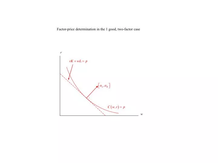
Factor-price determination in the 1 good, two-factor case. r. w. Factor-price determination in the 2x2 case (i). r. w. Factor-price determination in the 2x2 case (ii). r. w. Factor-price determination in the 2x2 case (iii). r. w. Factor-price determination in the 2x2 case (iv). r.

E N D
Factor-price determination in the 1 good, two-factor case r w
Factor-price determination in the 2x2 case (iv) r r(p) w w(p)
The Stolper-Samuelson theorem r r(p’) w w(p’)
The Lerner diagram (i) Step 1: set technologies and good prices unit-revenue isoquant K L
The Lerner diagram (ii) Step 2: determine profit-maximization points and factor prices unit-revenue isoquant K Profit-max. point for sector 1 1/r wL/y1 + rK/y1= 1 (unit isocost, common to both sectors) Profit-max. point for sector 2 -w/r L 1/w
The Lerner diagram (iii) Step 3: determine equilibrium factor intensities given factor prices unit-revenue isoquant K 1/r (w,r) wL/y1 + rK/y1= 1 (unit isocost) (w,r) -w/r L 1/w
The Lerner diagram (iv) Step 4: identify diversification cone K 1/r (w,r) This endowment can be fully employed by a linear combination of industries 1 and 2’s factor intensities: in the DC wL/y1 + rK/y1= 1 (w,r) This one can’t: out of the DC -w/r L 1/w
The Lerner diagram with everything in it unit-revenue isoquant K 1/r (w,r) wL/y1 + rK/y1= 1 (unit isocost) Profit-max. point for sector 1 (w,r) Profit-max. point for sector 2 -w/r L 1/w
The Rybczynski Theorem K Home capital endowment V2’ V2 Home diversification cone V1’ = V2’ L O Home labor endowment
The factor-price equalization set K O’ L* Home capital endowment V2 Home diversification cone = V2 V1 L O Home labor endowment K*
Factor-price determination in the 2x2 case: Factor-intensity reversal More flexible technology r In this cone, both industries are more labor intensive than in the other one w
The factor content of production and consumption K O’ L* Home capital endowment (home is cap-abundant) Fi(factor content of trade) Vi(production) ADi = Vi - Fi(consumption) L O Home labor endowment K*
The factor content of production and consumption: Trade surplus K O’ L* Home capital endowment Vi(production) ADi = Vi - Fi(consumption) L O Home labor endowment K*
Rybczynski effect in goods space y2 “Rybczynski expansion path” y1
L y y y time time time Apparel Textiles Textile Machinery Chemicals K B Leontieff isoquants A Time path of capital accumulation Apparel y Machinery time Chemicals
Intra-industry specialization Portable radios Satellites y time k1 k2 k3 k3
Stolper-Samuelson effects wS/wU Autarky wS/wU Skill premium under autarchy No FPE set H/L Skill premium after liberalization H/L FPE set
LA’s liberalization vs. Asia’s: Wood’s argument wS/wU wS/wU Skill premium under autarchy H/L LA in the 90s Asia in the 70s Skill premium after liberalization H/L FPE set before the big 5’s entry FPE set after the big 5’s entry
Defensive skill-biased technical change (Thoenig-Verdier) α (proportion of low-tech firms) Defensive technical change E0 α0 “No-bias condition” VS up R&D sector’s resource constraint (unit hazard rate of innovations) 0 V1 down meaning “per sector” (look at R&D resource constraint)
Defensive skill-biased technical change (Thoenig-Verdier) α (proportion of low-tech firms) after trade E0 E1 α0 E2 “No-bias condition”: unaffected by trade opening α1 before trade R&D sector’s resource constraint: shifts up with trade opening (unit hazard rate of innovations) 0 1 2
Offshoring with a continuum of goods unit costs C*(.) C*’(.) C’(.) C(.) E1 E0 Production migrating to the South Production staying in the North i
Inverse demand pm MR MC + TC (for the foreign firm) MC
Monopolistic competition: fixed markup 1/ zero-profit condition markup c (consumption per head) Consumers’ budget constraint n
Monopolistic competition: variable markup 1/ zero-profit condition markup c (consumption per head) Consumers’ budget constraint n
Figure 5.1 OLS estimate Elasticity to estimate (constant and common to all firms) firm 1 firm 2 firm 1 firm 2 no exports