Download
1 / 34
380 likes | 612 Views
GARCH and VaR. Downloads. Today’s work is in: matlab_lec05.m Functions we need today: simGARCH.m, simsecSV.m Datasets we need today: data_msft.m. GARCH(1,1). Assume returns follow: Where ε t is i.i.d. standard normal and µ=0 Zero mean is not a bad assumption for daily data

E N D
Downloads • Today’s work is in: matlab_lec05.m • Functions we need today: simGARCH.m, simsecSV.m • Datasets we need today: data_msft.m
GARCH(1,1) • Assume returns follow: • Where εt is i.i.d. standard normal and µ=0 • Zero mean is not a bad assumption for daily data • We saw that moving averages of r2 and σ2 look very similar for daily data • Don’t need µ=0 but it makes math easier
Simulating GARCH %this function simulates GARCH(1,1) w/ params w,a,b %output is Tx2 matrix with r in 1st column, sigmasq in 2nd function out=simGARCH(w,a,b,T); r=zeros(T+100,1); sigmasq=zeros(T+100,1); r(1)=0; sigmasq(1)=w/(1-a-b); for t=1:T-1+100; r(t+1)=randn(1)*sqrt(sigmasq(t)); sigmasq(t+1)=w+a*(r(t+1)^2)+b*sigmasq(t); end; out=[r(101:T+100) sigmasq(101:T+100)];
Simulating GARCH %simulate and look at output >>w=.05; a=.1; b=.8; T=1000; >>out=simGARCH(w,a,b,T); >>subplot(3,1,1); plot(out(:,1)); >>title('r'); >>subplot(3,1,2); plot(out(:,1).^2); >>title('r^{2}'); >>subplot(3,1,3); plot(out(:,2)); >>title('\sigma^{2}');
Estimating GARCH • We can now simulate GARCH(1,1)! • However what we really care about is knowing today’s volatility σt • We cannot observe σt in the data; we only observe rt • Simulation does not really help • How to find σt from rt? • If we know ω, α, and β we can estimate σt from rt • How to find ω, α, and β ?
Estimating GARCH • Note that E[rt+12]=σt2 and we can always write rt+12=E[rt+12]+zt+1=σt2+zt+1 where zt+1 is some zero mean variable
Estimating GARCH • GARCH(1,1) implies: • We can regress rt2 on its lags: • Now we can use coefficients of regression to find out ω, α, and β
Estimating GARCH >>w=.05; a=.1; b=.8; T=100000; out=simGARCH(w,a,b,T); >>clear X; n=100; >>for i=1:n; X(:,i)=out(n-i+1:T-i,1).^2; end; >>Y=out(n+1:T,1).^2; >>regcoef=regress(Y,[ones(T-n,1) X]); >>aest=regcoef(2); >>best=regcoef(3)/regcoef(2); >>west=regcoef(1)/((1-best^n)/(1-best)); >>disp([w a b; west aest best]); >> 0.0500 0.1000 0.8000 0.0517 0.0973 0.8024
Estimating GARCH • Note that we only used A1 and A2 to find α and β, however all of the other equations must hold as well • These are called over-identifying restrictions • If T was very large each equation would hold exactly • Because of estimation error the other equations only hold approximately
Estimating GARCH • We can see how well they hold: >>subplot; >>plot(a*b.^[0:8],regcoef(2:10),'.'); hold on; >>plot(regcoef(2:10),regcoef(2:10),'k') %all points should line up along the 45 degree line • There are more efficient ways of estimating GARCH using more equations • Using A1 and A2 only is less efficient, but still unbiased and works well if T is large enough
Estimating GARCH • Matlab has functions that use more efficient (and slower) methods to estimate GARCH • function ugarch(r,p,q) estimates garch(p,q) on the timeseries r • p and q are the lags on variance and squared returns terms in GARCH(p,q) • We are using p=1, q=1 • The output is [ωβα] • Note the different order from our convention
>>[w b a]=ugarch(out(:,1),1,1) %%%%%%%%%%%%%%%%%%%%%%%%%%%%%%%%%%%%%%%%%%%%%%%%%%%%%%%%%%% Diagnostic Information Number of variables: 3 Functions Objective: ugarchllf Gradient: finite-differencing Hessian: finite-differencing (or Quasi-Newton) Constraints Nonlinear constraints: do not exist Number of linear inequality constraints: 1 Number of linear equality constraints: 0 Number of lower bound constraints: 3 Number of upper bound constraints: 0 Algorithm selected medium-scale %%%%%%%%%%%%%%%%%%%%%%%%%%%%%%%%%%%%%%%%%%%%%%%%%%%%%%%%%%% End diagnostic information Max Line search Directional First-order Iter F-count f(x) constraint steplength derivative optimality Procedure 0 4 104763 -0.0493 1 12 104473 -0.04622 0.0625 2.49e+003 3.35e+004 2 24 104473 -0.04789 0.00391 1.99e+003 5.24e+003 3 33 104458 -0.06058 0.0313 343 2.39e+003 4 40 104458 -0.05415 0.125 93.8 4.9e+003 5 47 104456 -0.04748 0.125 48.4 1.5e+003 6 51 104453 -0.05498 1 4.8 1.06e+003 7 55 104452 -0.05318 1 -0.0914 30.1 8 59 104452 -0.05291 1 0.000356 2.79 9 63 104452 -0.05292 1 2.75e-007 0.132 Optimization terminated: magnitude of directional derivative in search direction less than 2*options.TolFun and maximum constraint violation is less than options.TolCon. No active inequalities. >> disp([w a b]) 0.0529 0.1016 0.7913
Estimating GARCH • Now lets estimate GARCH(1,1) on (i) Microsoft data (ii) simulated data with stochastic volatility (with parameters calibrated to Microsoft) • Note that the simulated data does not come from a GARCH model but does come from a different model with predictable volatility • GARCH is just a convenient way to estimate volatility
Data >>data_msft; >>rmsft=msft(:,4); >>sigma=std(rmsft); mu=mean(rmsft)-.5*sigma^2; T=length(rmsft); >>timeline=round(msft(1,2)/10000)+(round(msft(T,2)/10000)-round(msft(1,2)/10000))*([1:T]-1)/(T-1); >>nlow=sum(rmsft<-.1); >>nhigh=sum(rmsft>.1); >>p1=nlow/T; p2=nhigh/T; >>J1=-.15; J2=.15; >>sigmaS=.0025; rho=.96; >>rsim=simsecSV(mu,sigma,J1,J2,p1,p2,rho,sigmaS,T); >>subplot(2,1,1); plot(timeline,rmsft(1:T)); >>title('MSFT'); axis([timeline(1) timeline(T) -.2 .2]); >>subplot(2,1,2); plot(timeline,rsim(1:T)); >>title('Simulated'); axis([timeline(1) timeline(T) -.2 .2]);
Estimating GARCHMSFT >>n=100; clear X; >>for i=1:n; X(:,i)=rmsft(n-i+1:T-i,1).^2; >>end; >>Y=rmsft(n+1:T,1).^2; >>regcoef=regress(Y,[ones(T-n,1) X]); >>a=regcoef(2); >>b=regcoef(3)/regcoef(2); >>w=regcoef(1)/((1-b^n)/(1-b)); >>disp([w a b]); 0.0000 0.0558 0.9241 %Note strong evidence of persistence in volatility
Estimating GARCHSimulated DATA >>n=100; clear X; >>for i=1:n; X(:,i)=rsim(n-i+1:T-i,1).^2; >>end; >>Y=rsim(n+1:T,1).^2; >>regcoefS=regress(Y,[ones(T-n,1) X]); >>asim=regcoefS(2); >>bsim=regcoefS(3)/regcoefS(2); >>wsim=regcoefS(1)/((1-bsim^n)/(1-bsim)); >>disp([wsim asim bsim]); 0.0000 0.0623 0.9604
OveridentifyingRestrictions subplot; plot(a*b.^[0:8],regcoef(2:10),'sb','MarkerSize',10); hold on; plot(asim*bsim.^[0:8],regcoefS(2:10),'ro','MarkerSize',10); plot(regcoef(2:10),regcoef(2:10),'k'); xlabel('Coefficients implied by \alpha, \beta'); ylabel('Actual coefficients'); legend('MSFT','Simulated');
Estimating Volatility:MSFT >>vmsft=zeros(T,1); >>n=100; >>for t=n+1:T; k=0; s=0; for i=1:n; k=k+b^(i-1); s=s+(rmsft(t-i)^2)*b^(i-1); end; vmsft(t)=sqrt(w*k+a*s); end; >>vmsft(1:n)=mean(vmsft(n+1:T)); >>subplot(2,1,1); plot(timeline,rmsft(1:T)); >>title('MSFT Return'); axis([timeline(1) timeline(T) -.2 .2]); >>subplot(2,1,2); plot(timeline,vmsft(1:T)); >>title('MSFT Volatility'); axis([timeline(1) timeline(T) 0 .06]);
VaR • Value at Risk • Maximum loss not exceeded given a probability • The loss will be greater than rvar with probability pvar
Error Function • The error function is defined as: • The normal CDF gives the probability that a normally distributed variable is below some value, it can be rewritten in terms of the erf() • The inverse of a normal CDF gives the cut off value for the lowest p of the distribution, it can be rewritten in terms of the erf-1()
VaR >>T0=100000; sigma=.023; >>x=randn(T0,1)*sigma; >>rvar5=sqrt(2*sigma^2)*erfinv(2*.05-1); >>hist(x,50); axis([-.15 .15 0 8000]); hold on; >>plot(rvar5*ones(6,1),0:8000/5:8000,'r','LineWidth',3); >>disp([rvar5 sum(x<rvar5)/T0]); -0.0378 0.0504
GARCH VaR • If we believe that volatility changes through time, then VaR also changes through time • In particular if we believe GARCH, we can use GARCH to calculate today’s volatility and use it to predict value at risk • Note that we don’t have to use GARCH, we can use any volatility model we like • For example a simplistic model is constant volatility • We can then test whether the value at risk estimate was actually correct by comparing the total number of returns violating VaR(p) with the expected number of violations • The expected number of violations is p
GARCH VaR • Returns are normally distributed with volatility given by GARCH • Therefore rvar(t) will be a function of σ(t) just as before
MSFT VaR %%create VaR for GARCH(1,1) volatilty var5msft=sqrt(2*vmsft.^2)*erfinv(2*.05-1); %%plot MSFT volatility on top panel subplot(2,1,1); plot(timeline,vmsft); title('MSFT Volatility'); axis([timeline(1) timeline(T) 0 .06]); %%plot MSFT returns on lower panel subplot(2,1,2); plot(timeline,rmsft,'b'); hold on; %%on same panel plot MSFT VaR plot(timeline,var5msft,'r','LineWidth',3); title('MSFT VaR 5%'); axis([timeline(1) timeline(T) -.1 0]);
Back TestingVaR %compute fraction of times returns violate VaR disp('Percent Violations GARCH VaR 5%'); disp(sum(rmsft<var5msft)/T); %compute a constant volatility VaR for MSFT var5msftconstv=sqrt(2*std(rmsft).^2)*erfinv(2*.05-1); disp('Percent Violations Constant VolVaR 5%'); disp(sum(rmsft<var5msftconstv)/T); Percent Violations GARCH VaR 5% 0.0338 Percent Violations Constant VolVaR 5% 0.0344 %Note that both overestimate MSFT's number of extreme returns and therefore MSFT's risk