Download
1 / 17
190 likes | 387 Views
Single-Server Queue Model. Modeling and Simulation CS 313. Specification model.

E N D
Single-Server Queue Model Modeling and Simulation CS 313
Specification model The following variables, illustrated in Figure 1.2.2, provide the basis for moving from a conceptual model to a specification model. At their arrival to the service node, jobs are indexed by i = 1, 2, 3, … For each job there are six associated time variables.
Specification model (Arrivals) Rather than specifying the arrival times a1, a2, … explicitly, in some discrete-event simulation applications it is preferable to specify the arrival times r1, r2, …, thereby defining the arrival times implicitly, as shown:
Algorithmic question Given a knowledge of the arrival times a1, a2, ... (or, equivalently, the interarrival times r1, r2, ...), the associated service times s1, s2, ..., and the queue discipline, how can the delay times d1, d2, ... be computed? For some queue disciplines this question is more difficult to answer than for others. If the queue discipline is FIFO, however, then the answer is particularly simple. If the queue discipline is FIFO, di is determined by when ai occurs relative to ci−1.
Algorithmic question There are two cases to consider:
Algorithm The key point in algorithm development is that if the queue discipline is FIFO, then the truth of the expression ai < ci-1 determines whether or not job iwill experience a delay. An equation can be written for the delay that depends on the interarrival and service times only. That is:
Algorithm Algorithm 1.2.1 If the arrival times a1, a2,… and service times s1, s2,… are known, and if the server is initially idle, then this algorithm computes the delays d1, d2,… in a single-server FIFO service node with infinite capacity.
Algorithm Algorithm 1.2.1 The GetArrival and GetService procedures read the next arrival and service time from a file. Example: Algorithm 1.2.1 used to process n = 10 jobs
Output statistics • The purpose of simulation is insight gained by looking at statistics. • The importance of various statistics varies on perspective: • Job perspective: wait time is most important • Manager perspective: utilization is critical • Statistics are broken down into two categories: • Job-averaged statistics • Time-averaged statistics
Job-Averaged Statistics • Job-averaged statistics: computed via typical arithmetic mean • Average interarrival time: • The reciprocal of the average interarrival time, , is the arrival rate; • Average service time: • The reciprocal of the average service time, , is the service rate.
Output statistics • For the 10 jobs in the previous example: • Average interarrival time is: • The server is not quite able to process jobs at the rate they arrive on average.
Job-Averaged statistics The average delay and average wait are defined as: Recall wi = di + si for all i The point here is that it is sufficient to compute any two of the statistics . . The third statistic can then be computed from the other two, if appropriate.
Job-Averaged statistics From the data in the previous example: Therefore: Recall verification is one (difficult) step of model development Consistency check: used to verify that a simulation satisfies known equations:
Time-Averaged statistics • Time-averaged statistics: defined by area under a curve (integration) • For SSQ, need three additional functions: • l (t): number of jobs in the service node at time t • q(t): number of jobs in the queue at time t • x(t): number of jobs in service at time t. • By definition, l (t) = q(t) + x(t) • l (t) = 0, 1, 2, . . . • q(t) = 0, 1, 2, . . . • x(t) = 0, 1
Time-averaged statistics • All three functions are piece-wise constant • Figures for q(·) and x(·) can be deduced • q(t) = 0 and x(t) = 0 if and only if l(t) = 0
Time-Averaged statistics Over the time interval (0, T ): Since l (t) = q(t) + x(t) for all t > 0 Sufficient to calculate any two of
Time-Averaged statistics The average of numerous random observations (samples) of the number in the service node should be close to Same holds for Server utilization: time-averaged number in service also represents the probability the server is busy.