Download

1 / 34
350 likes | 485 Views
The Chi-square test is used to analyze counts of categorical data with three types: goodness of fit, independence, and homogeneity. The test relies on Chi-square distributions, making assumptions like random sampling and adequate sample sizes. Learn how to conduct Chi-square tests for different scenarios, interpret results, and formulate hypotheses correctly. Discover practical examples and understand why the Chi-square goodness-of-fit test might not be suitable in certain situations.

E N D
Chi-square test • Used to test the counts of categorical data • Three types • Goodness of fit (univariate) • Independence (bivariate) • Homogeneity (univariate with two samples)
c2 distribution • Different df have different curves • Skewed right • As df increases, curve shifts toward right & becomes more like a normal curve
c2 assumptions • SRS – reasonably random sample • Have countsof categorical data & we expect each category to happen at least once • Sample size – to insure that the sample size is large enough we should expect at least five in each category. ***Be sure to list expected counts!! Combine these together: All expected counts are at least 5.
c2 Goodness of fit test • Uses univariate data • Want to see how well the observedcounts “fit” what we expect the counts to be • Use c2cdf function on the calculator to find p-values Based on df – df = number of categories - 1
Hypotheses – written in words H0: proportions are equal Ha: at least one proportion is not the same Be sure to write in context!
Example: Does the color of a car influence the chance that it will be stolen? Of 830 cars reported stolen, 140 were white, 100 were blue, 270 were red, 230 were black, and 90 were other colors. It is known that 15% of all cars are white, 15% are blue, 35% are red, 30% are black, and 5% are other colors.
Let π1, π2, . . . Π5 denote true proportions of stolen cars that fall into the 5 color categories Ho: π1 = .15, π2 = .15, π3 = .35, π4 = .30, π5 = .05 (The proportion of each color of stolen cars is the same as the proportion of colors of cars) Ha; Ho is not true. (The proportion of each color of stolen cars is not the same as the proportion of colors of cars) α = .01 Test statistic: Assumptions: The sample was a random sample of stolen cars. All expected counts are greater than 5, so the sample size is large enough to use the chi-square test.
Calculations: = 1.93 + 4.82 + 1.45 + 1.45 + 56.68 = 66.33 P-value: x2cdf(66.33,∞, 4) ≈ 0 Because P-value < α, Ho is rejected. There is convincing evidence that at least one of the color proportions for stolen cars differs from the corresponding proportion for all cars.
A company says its premium mixture of nuts contains 10% Brazil nuts, 20% cashews, 20% almonds, 10% hazelnuts and 40% peanuts. You buy a large can and separate the nuts. Upon weighing them, you find there are 112 g Brazil nuts, 183 g of cashews, 207 g of almonds, 71 g or hazelnuts, and 446 g of peanuts. You wonder whether your mix is significantly different from what the company advertises? Why is the chi-square goodness-of-fit test NOT appropriate here? What might you do instead of weighing the nuts in order to use chi-square? Because we do NOT have counts of the type of nuts. We could count the number of each type of nut and then perform a c2 test.
c2 test for independence • Used with categorical, bivariate data from ONEsample • you have two characteristics of a population, and you want to see if there is any association between the characteristics(2 variables, 1 population)
Assumptions & formula remain the same! Hypotheses – written in words H0: two variables are independent Ha: two variables are dependent Be sure to write in context!
Degrees of freedom Or cover up one row & one column & count the number of cells remaining!
A claim is made regarding the independence of the data. Ho: there is not association between gender of lifestyle choice, the variables are independent Ha: there is an association between gender of lifestyle choice, the variables are dependent Verify the requirements for the chi-square test for independence are satisfied. (1) data is randomly selected (2) all expected cell counts are greater than or equal to 5.
Calculate the expected frequencies (counts) for each cell in the contingency table. Observed Counts Expected Counts
36.84 P-value = 0.00000001 with 2 df Since p-value is less than significance level, I would reject the null hypothesis. The data is statistically significant and I am led to believe that there is an association between gender and lifestyle choice and that these variables are dependent
c2 test for homogeneity • Used with a single categorical variable from two (or more) independent samples • Used to see if the two populations are the same (homogeneous) • (1 variable, multiple populations)
Assumptions & formula remain the same! Expected counts & df are found the same way as test for independence. Only change is the hypotheses!
Hypotheses – written in words H0: the proportions for the two (or more) distributions are the same Ha: At least one of the proportions for the distributions is different Be sure to write in context!
EXAMPLE A Test of Homogeneity of Proportions The following question was asked of a random sample of individuals in 1992, 1998, and 2001: “Would you tell me if you feel being a teacher is an occupation of very great prestige?” The results of the survey are presented below:
A claim is made regarding the homogeneity of the data. Ho: the proportions of individuals who feel teaching is an occupation of very great prestige in each year are equal Ha: the proportions of individuals who feel teaching is an occupation of very great prestige in each year are not equal
Calculate the expected frequencies (counts) for each cell in the contingency table. Observed Counts Expected Counts
Step 3: Verify the requirements for the chi-square test for homogeneity are satisfied. (1) data is randomly selected (2) all expected cell counts are greater than or equal to 5. 2.26 p-value = 0.3228 with 2 df Since p-value is greater than any significance level, I would fail to reject the null hypothesis. The data is not statistically significant and I can not conclude that the proportions of individuals who feel teaching is an occupation of very great prestige is different each year
Linear Regression Inference Inference for Linear Regression • Is there really a linear relationship between x and y in the population, or could the pattern we see in the scatterplot plausibly happen just by chance? • In the population, how much will the predicted value of y change for each increase of 1 unit in x? What’s the margin of error for this estimate?
You should always check the conditions before doing inference about the regression model. Although the conditions for regression inference are a bit complicated, it is not hard to check for major violations. Start by making a histogram or Normal probability plot of the residuals and also a residual plot. Here’s a summary of how to check the conditions one by one. Inference for Linear Regression • How to Check the Conditions for Inference How to Check the Conditions for Regression Inference • Linear Examine the scatterplot to check that the overall pattern is roughly linear. Look for curved patterns in the residual plot. Check to see that the residuals center on the “residual = 0” line at each x-value in the residual plot. • Independent Look at how the data were produced. Random sampling and random assignment help ensure the independence of individual observations. If sampling is done without replacement, remember to check that the population is at least 10 times as large as the sample (10% condition). • Normal Make a stemplot, histogram, or Normal probability plot of the residuals and check for clear skewness or other major departures from Normality. • Equal variance Look at the scatter of the residuals above and below the “residual = 0” line in the residual plot. The amount of scatter should be roughly the same from the smallest to the largest x-value. • Random See if the data were produced by random sampling or a randomized experiment. L I N E R
Mrs. Barrett’s class did a variation of the helicopter experiment on page 738. Students randomly assigned 14 helicopters to each of five drop heights: 152 centimeters (cm), 203 cm, 254 cm, 307 cm, and 442 cm. Teams of students released the 70 helicopters in a predetermined random order and measured the flight times in seconds. The class used Minitab to carry out a least-squares regression analysis for these data. A scatterplot, residual plot, histogram, and Normal probability plot of the residuals are shown below. Inference for Linear Regression • Example: The Helicopter Experiment • Linear The scatterplot shows a clear linear form. For each drop height used in the experiment, the residuals are centered on the horizontal line at 0. The residual plot shows a random scatter about the horizontal line. • Normal The histogram of the residuals is single-peaked, unimodal, and somewhat bell-shaped. In addition, the Normal probability plot is very close to linear. • Independent Because the helicopters were released in a random order and no helicopter was used twice, knowing the result of one observation should give no additional information about another observation. • Equal variance The residual plot shows a similar amount of scatter about the residual = 0 line for the 152, 203, 254, and 442 cm drop heights. Flight times (and the corresponding residuals) seem to vary more for the helicopters that were dropped from a height of 307 cm. • Random The helicopters were randomly assigned to the five possible drop heights. Except for a slight concern about the equal-variance condition, we should be safe performing inference about the regression model in this setting.
Computer output from the least-squares regression analysis on the helicopter data for Mrs. Barrett’s class is shown below. Inference for Linear Regression • Example: The Helicopter Experiment The slope β of the true regression line says how much the average flight time of the paper helicopters increases when the drop height increases by 1 centimeter. Because b = 0.0057244 estimates the unknown β, we estimate that, on average, flight time increases by about 0.0057244 seconds for each additional centimeter of drop height. We need the intercept a = -0.03761 to draw the line and make predictions, but it has no statistical meaning in this example. No helicopter was dropped from less than 150 cm, so we have no data near x = 0. We might expect the actual y-intercept α of the true regression line to be 0 because it should take no time for a helicopter to fall no distance. The y-intercept of the sample regression line is -0.03761, which is pretty close to 0. Our estimate for the standard deviation σ of flight times about the true regression line at each x-value is s = 0.168 seconds. This is also the size of a typical prediction error if we use the least-squares regression line to predict the flight time of a helicopter from its drop height.
What happens if we transform the values of b by standardizing? Since the sampling distribution of b is Normal, the statistic has the standard Normal distribution. Inference for Linear Regression • The Sampling Distribution of b Replacing the standard deviation σbof the sampling distribution with its standard error gives the statistic which has a t distribution with n - 2 degrees of freedom. The figure shows the result of standardizing the values in the sampling distribution of b from the Old Faithful example. Recall, n = 20 for this example. The superimposed curve is a t distribution with df = 20 – 2 = 18.
Inference for Linear Regression • Constructing a Confidence Interval for the Slope The slope β of the population (true) regression line µy = α + βx is the rate of change of the mean response as the explanatory variable increases. We often want to estimate β. The slope b of the sample regression line is our point estimate for β. A confidence interval is more useful than the point estimate because it shows how precise the estimate b is likely to be. The confidence interval for β has the familiar form statistic ± (critical value) · (standard deviation of statistic) Because we use the statistic b as our estimate, the confidence interval is b±t* SEb We call this a t interval for the slope. t Interval for the Slope of a Least-Squares Regression Line When the conditions for regression inference are met, a level C confidence interval for the slope βof the population (true) regression line is b±t* SEb In this formula, the standard error of the slope is and t* is the critical value for the t distribution with df = n - 2 having area C between -t* and t*.
Inference for Linear Regression • Example: Helicopter Experiment Earlier, we used Minitab to perform a least-squares regression analysis on the helicopter data for Mrs. Barrett’s class. Recall that the data came from dropping 70 paper helicopters from various heights and measuring the flight times. We checked conditions for performing inference earlier. Construct and interpret a 95% confidence interval for the slope of the population regression line. SEb = 0.0002018, from the “SE Coef ” column in the computer output. Because the conditions are met, we can calculate a t interval for the slope β based on a t distribution with df = n - 2 = 70 - 2 = 68. Using the more conservative df = 60 from Table Bgives t* = 2.000. The 95% confidence interval is b ± t* SEb = 0.0057244 ± 2.000(0.0002018) = 0.0057244 ± 0.0004036 = (0.0053208, 0.0061280) We are 95% confident that the interval from 0.0053208 to 0.0061280 seconds per cm captures the slope of the true regression line relating the flight time y and drop height x of paper helicopters.
Inference for Linear Regression • Example: Crying and IQ Do: With no obvious violations of the conditions, we proceed to inference. The test statistic and P-value can be found in the Minitab output. The Minitab output gives P = 0.004 as the P-value for a two-sided test. The P-value for the one-sided test is half of this, P = 0.002. Conclude: The P-value, 0.002, is less than our α = 0.05 significance level, so we have enough evidence to reject H0and conclude that there is a positive linear relationship between intensity of crying and IQ score in the population of infants.