Download
1 / 18
180 likes | 313 Views
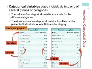
Categorical Data. Contingency Tables represent the association between two or more qualitative or categorical variables. Example of females in San Francisco:. We can express these numbers in frequency terms by dividing each number by the grand total of 1075. 26/1075 = .024 or 2.4%.

E N D
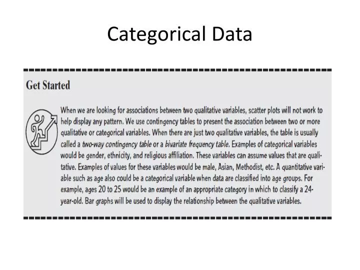
Contingency Tables represent the association between two or more qualitative or categorical variables. Example of females in San Francisco:
We can express these numbers in frequency terms by dividing each number by the grand total of 1075 26/1075 = .024 or 2.4% 422/1075 = .393 or 39.3% 144/1075 = .134 or 13.4% Note the individual values, age subtotals, and ethnicity subtotals all add to 100%.
Marginal Distributions Marginal Distributions show the frequency distribution of one variable relative to the grand total. In the previous example, the green subtotal is the marginal distribution for ethnicity, and the purple subtotal is the marginal distribution for age. Note that the marginal distributions are the distributions you would have if you only had information on ethnicity, or on age.
Conditional Distributions Conditional Distributions show the relative frequencies (which must sum to 100%) of one variable, knowing the value of the other variable. Mathematically, conditional distributions are found by dividing the individual data by the known row or column value.
Example: If you know the person is white, the marginal frequency distribution is… 26/415 = .063 or 6.3% Just convert the “white” ethnicity column into percentages, and ignore all other data.
More generally, if you know the person’s ethnicity, whether it is white, black or hispanic, the marginal distributions are…
Similarly, we can get conditional distributions given we know the person’s age category:
Dependent and Independent Variables Categorical variables are said to be independent if one variable has no effect on the frequency distribution of the other variable. Mathematically, the marginal distributions are the same, regardless of the value of the (independent) variable. Counter-Example of dependent variables: Pregnancy, Age, and Gender. Questions: If it is true that, at any time, 2.1% of the total population is pregnant, does that mean that 2.1% of men are pregnant? What about 2 year old baby girls? Of course, neither men (of any age) nor baby girls can be pregnant. On the other hand, for young lades between 16 and 40 years old, the percentage that are pregnant is much higher than 2.1%.
Textbook example of independent variables Is the probability (frequency) of a student giving the College President a “favorable” or “unfavorable” rating different, depending upon whether the student is a male or female?
Example of Independent Variables Question: If you know that the rating was a male (or female), can you better guess what the student’s opinion was? Remember, 54/75 = .72 or 72%, etc. Question: If you know that the rating was favorable (or unfavorable), can you better guess if it was a male or female student giving an opinion? Remember, 54/72 = .75 or 75%, etc.
When viewed major-by-major, the acceptance rates seem to favor females. IF FEMALES ARE DISCRIMINATED AGAINST, HOW CAN THAT BE?
In this study, 52% of males, but only 39% of females, were accepted. What is going on? These tables are calculating marginal frequencies downward These tables are calculating marginal frequencies across The top table asks, given the major, what percentage of males, and what percentage of females, are being accepted. The bottom table asks, given that it’s a male or female, which majors are the students applying for, and at what rate are they being admitted.
Easy to get accepted Hard to get accepted Females were getting accepted less overall because they were applying for the most difficult majors to get accepted into, regardless of whether the student was a male or female!
In this example, the problem is not discrimination against females. Though they are trying to go to the same university, the females are trying to get into much more difficult majors than the males are. That is why they succeed less often. If you would treat each major as a separate school (which, functionally, it is!) then there would be no appearance of discrimination! Maybe we should try using the door instead of the window! Just like the boys! Crash! Ouch! Girls, why aren’t you going in to school? But look at all the boys in there. They just don’t like us because we’re girls! Wah! Wah! Wah! Boom! Oh! Uh! Sorry. I thought you were going in. Because the window is locked. Anyway, it’s too small! Ugh! Ow!