Download
1 / 27
270 likes | 273 Views
This overview discusses the use of ground-based radar and lidar to evaluate model clouds, including identifying targets in radar and lidar data, evaluating cloud fraction and water content, and forecasting skill scores. It also highlights the Cloudnet methodology and the evaluation of cloud variables in forecast and climate models.

E N D
Use of ground-based radar and lidar to evaluate model clouds Robin Hogan Ewan O’Connor Julien Delanoe Anthony Illingworth
Overview • Cloud radar and lidar sites worldwide • Cloud evaluation over Europe as part of Cloudnet • Identifying targets in radar and lidar data (cloud droplets, ice particles, drizzle/rain, aerosol, insects etc) • Evaluation of cloud fraction • Liquid water content • Ice water content • Forecast evaluation using skill scores • Drizzle rates beneath stratocumulus • The future: variational methods • Optimal combination of many instruments
Continuous cloud-observing sites AMF shortly to move to Southern Germany for COPS • Key cloud instruments at each site: • Radar, lidar and microwave radiometers
The Cloudnet methodologyRecently completed EU project; www.cloud-net.org • Aim: to retrieve and evaluate the crucial cloud variables in forecast and climate models • Models: Met Office (4-km, 12-km and global), ECMWF, Météo-France, KNMI RACMO, Swedish RCA model, DWD • Variables: target classification, cloud fraction, liquid water content, ice water content, drizzle rate, mean drizzle drop size, ice effective radius, TKE dissipation rate • Sites: 4 Cloudnet sites in Europe, 6 ARM including the mobile facility • Period: Several years near-continuous data from each site • Crucial aspects • Common formats (including errors & data quality flags) allow all algorithms to be applied at all sites to evaluate all models • Evaluate for months and years: avoid unrepresentative case studies
First step: target classification Ice Liquid Rain Aerosol Insects • Combining radar, lidar and model allows the type of cloud (or other target) to be identified • From this can calculate cloud fraction in each model gridbox Example from US ARM site: Need to distinguish insects from cloud
Cloud fraction Observations Met Office Mesoscale Model ECMWF Global Model Meteo-France ARPEGE Model KNMI RACMO Model Swedish RCA model
Cloud fraction in 7 models • Uncertain above 7 km as must remove undetectable clouds in model • All models except DWD underestimate mid-level cloud; some have separate “radiatively inactive” snow (ECMWF, DWD); Met Office has combined ice and snow but still underestimates cloud fraction • Wide range of low cloud amounts in models • Mean & PDF for 2004 for Chilbolton, Paris and Cabauw 0-7 km Illingworth, Hogan, O’Connor et al., submitted to BAMS
A change to Meteo-France cloud scheme • Compare cloud fraction to observations before and after April 2003 • Note that cloud fraction and water content are entirely diagnostic But human obs. indicate model now underestimates mean cloud-cover! Compensation of errors: overlap scheme changed from random to maximum-random beforeafter April 2003
Liquid water content • Met Office mesoscale tends to underestimate supercooled water occurrence • ECMWF has far too great an occurrence of low LWC values • KNMI RACMO identical to ECMWF: same physics package! • LWC derived using the scaled adiabatic method • Lidar and radar provide cloud boundaries, adiabatic LWC profile then scaled to match liquid water path from microwave radiometers 0-3 km
Ice water content • ECMWF and Met Office within the observational errors at all heights • Encouraging: AMIP implied an error of a factor of 10! • IWC estimated from radar reflectivity and temperature • Rain events excluded from comparison due to mm-wave attenuation • For IWC above rain, use cm-wave radar (e.g. Hogan et al., JAM, 2006) 3-7 km • Be careful in interpretation: mean IWC dominated by occasional large values so PDF more relevant for radiative properties
Contingency tables Model cloud Model clear-sky Comparison with Met Office model over Chilbolton October 2003 Observed cloud Observed clear-sky
Equitable threat score • Definition: ETS = (A-E)/(A+B+C-E) • E removes those hits that occurred by chance • 1 = perfect forecast, 0 = random forecast • Measure of the skill of forecasting cloud fraction>0.05 • Assesses the weather of the model not its climate • Persistence forecast is shown for comparison • Lower skill in summer convective events
Drizzle! • Radar and lidar used to derive drizzle rate below stratocumulus • Important for cloud lifetime in climate models O’Connor et al. (2005) • Met Office uses Marshall-Palmer distribution for all rain • Observations show that this tends to overestimate drop size in the lower rain rates • Most models (e.g. ECMWF) have no explicit raindrop size distribution
1-year comparison with models • ECMWF, Met Office and Meteo-France overestimate drizzle rate • Problem with auto-conversion and/or accretion rates? • Larger drops in model fall faster so too many reach surface rather than evaporating: drying effect on boundary layer? Met Office ECMWF model Observations O’Connor et al., submitted to J. Climate
Variational retrieval • The retrieval guy’s dream is to do everything variationally: • Make a first guess of the profile of cloud properties • Use forward models to predict observations that are available (e.g. radar reflectivity, Doppler velocity, lidar backscatter, microwave radiances, geostationary TOA infrared radiances) and the Jacobian • Iteratively refine the cloud profile to minimize the difference between the observations and the forward model in a least-squares sense • Existing methods only perform retrievals where both the radar and lidar detect the cloud • A variational method (1D-VAR) can spread information vertically to regions detected by just the radar or the lidar • We have done this for ice clouds (liquid clouds to follow) • Use fast lidar multiple scattering model that incorporates high orders of scattering (Hogan, Appl. Opt., 2006) • Use the two-stream source function method for the SEVIRI radiances • Use extinction coefficient and “normalized number concentration parameter” as the state variables…
Radar forward model and a priori • Create lookup tables • Gamma size distributions • Choose mass-area-size relationships • Mie theory for 94-GHz reflectivity • Define normalized number concentration parameter N0* • “The N0 that an exponential distribution would have with same IWC and D0 as actual distribution” • Forward model predicts Z from the state variables (extinction and N0*) • Effective radius from lookup table • N0 has strong T dependence • Use Field et al. power-law as a-priori • When no lidar signal, retrieval relaxes to one based on Z and T (Liu and Illingworth 2000, Hogan et al. 2006) Field et al. (2005)
Lidar forward model: multiple scattering Wide field-of-view: forward scattered photons may be returned Narrow field-of-view: forward scattered photons escape • Degree of multiple scattering increases with field-of-view • Eloranta’s (1998) model • O (N m/m !) efficient for N points in profile and m-order scattering • Too expensive to take to more than 3rd or 4th order in retrieval (not enough) • New method: treats third and higher orders together • O (N 2) efficient • As accurate as Eloranta when taken to ~6th order • 3-4 orders of magnitude faster for N =50 (~ 0.1 ms) Ice cloud Molecules Liquid cloud Aerosol Hogan (Applied Optics, 2006). Code: www.met.rdg.ac.uk/clouds
Ice cloud: non-variational retrieval Donovan et al. (2000) Aircraft-simulated profiles with noise (from Hogan et al. 2006) • Existing algorithms can only be applied where both lidar and radar have signal Observations State variables Derived variables Retrieval is accurate but not perfectly stable where lidar loses signal
Variational radar/lidar retrieval • Noise in lidar backscatter feeds through to retrieved extinction Observations State variables Derived variables Lidar noise matched by retrieval Noise feeds through to other variables
…add smoothness constraint • Smoothness constraint: add a term to cost function to penalize curvature in the solution (J’ = l Sid2ai/dz2) Observations State variables Derived variables Retrieval reverts to a-priori N0 Extinction and IWC too low in radar-only region
…add a-priori error correlation • Use B (the a priori error covariance matrix) to smooth the N0 information in the vertical Observations State variables Derived variables Vertical correlation of error in N0 Extinction and IWC now more accurate
…add infrared radiances • Better fit to IWC and re at cloud top Observations State variables Derived variables Poorer fit to Z at cloud top: information here now from radiances
Example from the AMF in Niamey ARM Mobile Facility observations from Niamey, Niger, 22 July 2006 Also use SEVIRI channels at 8.7, 10.8, 12µm 94-GHz radar reflectivity 532-nm lidar backscatter
ResultsRadar+lidar only Retrieved visible extinction coefficient Retrievals in regions where only the radar or lidar detects the cloud Retrieved effective radius Preliminary results! By forward modelling radar instrument noise, we use the fact that a cloud is below the instrument sensitivity as a constraint 94-GHz radar reflectivity (forward model) 532-nm lidar backscatter (forward model)
Results Radar+lidar only Retrieved visible extinction coefficient Retrievals in regions where only the radar or lidar detects the cloud Retrieved effective radius Preliminary results! Large error where only one instrument detects the cloud Retrieval error in ln(extinction)
Results Radar, lidar, SEVERI radiances Retrieved visible extinction coefficient TOA radiances increase the optical depth and decrease particle size near cloud top Retrieved effective radius Preliminary results! Cloud-top error is greatly reduced Retrieval error in ln(extinction)
Future work • Ongoing Cloudnet-type evaluation of models • A large quantity of ARM data already processed • Would like to be able to evaluate model clouds in near real time (within a few days) to inform model update cycles • BUT need to establish continued funding for this activity! For quicklooks and further information: www.cloud-net.org • Variational retrieval method • Apply to more ground-based data • Apply to CloudSat/Calipso/MODIS (when Calipso data released) • New forward model including wide-angle multiple scattering for both radar and lidar • Evaluate ECMWF and Met Office models under CloudSat • Could form the basis for radar and lidar assimilation