Download
1 / 51
520 likes | 660 Views
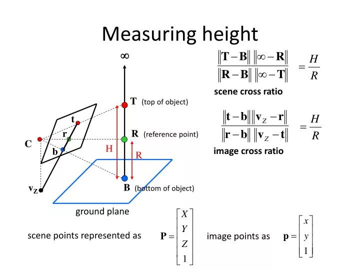
scene cross ratio. C. image cross ratio. Measuring height. . T (top of object). t. r. R (reference point). H. b. R. B (bottom of object). v Z. ground plane. scene points represented as. image points as. Measuring height. t. v. H. image cross ratio. v z. r.

E N D
scene cross ratio C image cross ratio Measuring height T (top of object) t r R (reference point) H b R B (bottom of object) vZ ground plane scene points represented as image points as
Measuring height t v H image cross ratio vz r vanishing line (horizon) t0 vx vy H R b0 b
3D Modeling from a photograph St. Jerome in his Study, H. Steenwick
3D Modeling from a photograph Flagellation, Piero della Francesca
3D Modeling from a photograph video by Antonio Criminisi
Camera calibration • Goal: estimate the camera parameters • Version 1: solve for projection matrix • Version 2: solve for camera parameters separately • intrinsics (focal length, principle point, pixel size) • extrinsics (rotation angles, translation) • radial distortion
= = similarly, π v , π v 2 Y 3 Z Vanishing points and projection matrix = vx (X vanishing point) Not So Fast! We only know v’s up to a scale factor • Can fully specify by providing 3 reference points
Calibration using a reference object • Place a known object in the scene • identify correspondence between image and scene • compute mapping from scene to image • Issues • must know geometry very accurately • must know 3D->2D correspondence
Estimating the projection matrix • Place a known object in the scene • identify correspondence between image and scene • compute mapping from scene to image
Alternative: multi-plane calibration Images courtesy Jean-Yves Bouguet, Intel Corp. • Advantage • Only requires a plane • Don’t have to know positions/orientations • Good code available online! (including in OpenCV) • Matlab version by Jean-Yves Bouget: http://www.vision.caltech.edu/bouguetj/calib_doc/index.html • Zhengyou Zhang’s web site: http://research.microsoft.com/~zhang/Calib/
Some Related Techniques • Image-Based Modeling and Photo Editing • Mok et al., SIGGRAPH 2001 • http://graphics.csail.mit.edu/ibedit/ • Single View Modeling of Free-Form Scenes • Zhang et al., CVPR 2001 • http://grail.cs.washington.edu/projects/svm/ • Tour Into The Picture • Anjyo et al., SIGGRAPH 1997 • http://koigakubo.hitachi.co.jp/little/DL_TipE.html
More than one view? • We now know all about the geometry of a single view • What happens if we have two cameras? What’s the transformation?
CS6670: Computer Vision Noah Snavely Lecture 10: Stereo Single image stereogram, by Niklas Een
Public Library, Stereoscopic Looking Room, Chicago, by Phillips, 1923
Mark Twain at Pool Table", no date, UCR Museum of Photography
Epipolar geometry epipolar lines (x2, y1) (x1, y1) Two images captured by a purely horizontal translating camera (rectified stereo pair) x2 -x1 = the disparity of pixel (x1, y1)
Stereo matching algorithms • Match Pixels in Conjugate Epipolar Lines • Assume brightness constancy • This is a tough problem • Numerous approaches • A good survey and evaluation: http://www.middlebury.edu/stereo/
For each epipolar line For each pixel in the left image Improvement: match windows Your basic stereo algorithm • compare with every pixel on same epipolar line in right image • pick pixel with minimum match cost
W = 3 W = 20 Window size • Better results with adaptive window • T. Kanade and M. Okutomi,A Stereo Matching Algorithm with an Adaptive Window: Theory and Experiment,, Proc. International Conference on Robotics and Automation, 1991. • D. Scharstein and R. Szeliski. Stereo matching with nonlinear diffusion. International Journal of Computer Vision, 28(2):155-174, July 1998
Stereo results • Data from University of Tsukuba • Similar results on other images without ground truth Scene Ground truth
Results with window search Window-based matching (best window size) Ground truth
Better methods exist... • State of the art method • Boykov et al., Fast Approximate Energy Minimization via Graph Cuts, • International Conference on Computer Vision, September 1999. Ground truth • For the latest and greatest: http://www.middlebury.edu/stereo/
Stereo as energy minimization • What defines a good stereo correspondence? • Match quality • Want each pixel to find a good match in the other image • Smoothness • If two pixels are adjacent, they should (usually) move about the same amount
Stereo as energy minimization • Expressing this mathematically • Match quality • Want each pixel to find a good match in the other image • Smoothness • If two pixels are adjacent, they should (usually) move about the same amount • We want to minimize • This is a special type of energy function known as an MRF (Markov Random Field) • Effective and fast algorithms have been recently developed: • Graph cuts, belief propagation…. • for more details (and code): http://vision.middlebury.edu/MRF/ • Great tutorials available online (including video of talks)
X z x x’ f f baseline C C’ Depth from disparity
Real-time stereo • Used for robot navigation (and other tasks) • Several software-based real-time stereo techniques have been developed (most based on simple discrete search) • Nomad robot searches for meteorites in Antartica • http://www.frc.ri.cmu.edu/projects/meteorobot/index.html
Stereo reconstruction pipeline • Steps • Calibrate cameras • Rectify images • Compute disparity • Estimate depth What will cause errors? • Camera calibration errors • Poor image resolution • Occlusions • Violations of brightness constancy (specular reflections) • Large motions • Low-contrast image regions
camera 1 camera 1 projector projector camera 2 Active stereo with structured light • Project “structured” light patterns onto the object • simplifies the correspondence problem Li Zhang’s one-shot stereo
Laser scanning • Optical triangulation • Project a single stripe of laser light • Scan it across the surface of the object • This is a very precise version of structured light scanning • Digital Michelangelo Project • http://graphics.stanford.edu/projects/mich/
Laser scanned models • The Digital Michelangelo Project, Levoy et al.
Laser scanned models • The Digital Michelangelo Project, Levoy et al.
Laser scanned models • The Digital Michelangelo Project, Levoy et al.
Laser scanned models • The Digital Michelangelo Project, Levoy et al.
Stereo as energy minimization • Find disparity map d that minimizes an energy function • Simple pixel / window matching = SSD distance between windows I(x, y) and J(x + d(x,y), y)
Stereo as energy minimization I(x, y) J(x, y) y = 141 d x C(x, y, d); the disparity space image (DSI)
Stereo as energy minimization y = 141 d x Simple pixel / window matching: choose the minimum of each column in the DSI independently:
Stereo as energy minimization • Better objective function { { smoothness cost match cost • Want each pixel to find a good match in the other image • Adjacent pixels should (usually) move about the same amount
Stereo as energy minimization match cost: smoothness cost: : set of neighboring pixels 4-connected neighborhood 8-connected neighborhood
Smoothness cost How do we choose V? L1 distance “Potts model”
Dynamic programming • Can minimize this independently per scanline using dynamic programming (DP) : minimum cost of solution such that d(x,y) = d
Dynamic programming • Finds “smooth” path through DPI from left to right y = 141 d x
Dynamic programming • Can we apply this trick in 2D as well? • No: dx,y-1 and dx-1,y may depend on different values of dx-1,y-1 Slide credit: D. Huttenlocher
Stereo as a minimization problem • The 2D problem has many local minima • Gradient descent doesn’t work well • And a large search space • n x m image w/ k disparities has knmpossible solutions • Finding the global minimum is NP-hard in general • Good approximations exist… we’ll see this soon