Download
1 / 59
590 likes | 594 Views
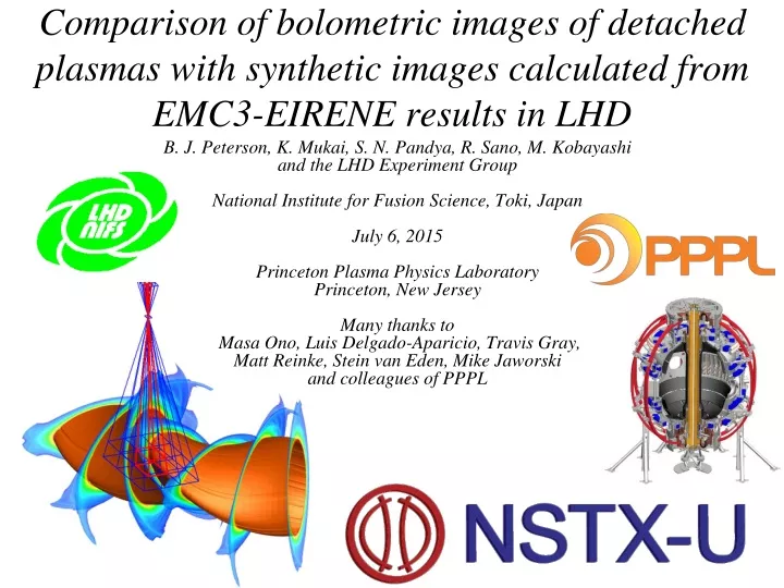
Comparison of bolometric images of detached plasmas with synthetic images calculated from EMC3-EIRENE results in LHD. B. J. Peterson, K. Mukai , S. N. Pandya , R. Sano, M. Kobayashi and the LHD Experiment Group National Institute for Fusion Science, Toki, Japan July 6, 2015

E N D
Comparison of bolometric images of detached plasmas with synthetic images calculated from EMC3-EIRENE results in LHD B. J. Peterson, K. Mukai, S. N. Pandya, R. Sano, M. Kobayashi and the LHD Experiment Group National Institute for Fusion Science, Toki, Japan July 6, 2015 Princeton Plasma Physics Laboratory Princeton, New Jersey Many thanks to Masa Ono, Luis Delgado-Aparicio, Travis Gray, Matt Reinke, Stein van Eden, Mike Jaworski and colleagues of PPPL
Outline • Introduction of Imaging Bolometer concept • SNR calculation • Foil thickness vs photon energy • Calibration • 2D tomography on JT-60U • 3D tomography on LHD • Comparison with synthetic images from EMC3-EIRENE during magnetic island detachment experiments • Design for NSTX-U • Conclusions ad future work B. J. Peterson PPPL seminar peterson@lhd.nifs.ac.jp 2015.7. 6
Outline • Introduction of Imaging Bolometer concept • SNR calculation • Foil thickness vs photon energy • Calibration • 2D tomography on JT-60U • 3D tomography on LHD • Comparison with synthetic images from EMC3-EIRENE during magnetic island detachment experiments • Design for NSTX-U • Conclusions ad future work B. J. Peterson PPPL seminar peterson@lhd.nifs.ac.jp 2015.7. 6
Concept - IR imaging Video Bolometer (IRVB) IR vacuum window vacuum vessel soft iron shield pin hole 1 m IR radiation Plasma Plasma radiation light shield tube vent IRcamera 1-5 mm Au, Pt, Ta foil (IR camera side is blackened with graphite plasma side left bare or blackened) IRVB copper frame (blackened with graphite) [1] B.J. Peterson, Rev. Sci. Instrum.70 (2000) 3696. [2] B.J. Peterson et al., Rev. Sci. Instrum.72 (2001) 923.
IRVB – Concept and Calibration Solve foil 2D heat diffusion equation for Prad IRVB pinhole camera copper frame IR measured by camera Plasma radiation absorbed by foil 2-D Laplacian thermal diffusivion to frame foil thermal diffusivity Thin foil light shield copper frame black body cooling term Terms to be calibrated plasma radiated power is determined by solving heat diffusion equation foil thermal conductivity bolometer pixel area foil thickness B.J. Peterson et al., Rev. Sci. Instrum.74 (2003) 2040.
Outline • Introduction of Imaging Bolometer concept • SNR calculation • Foil thickness vs photon energy • Calibration • 2D tomography on JT-60U • 3D tomography on LHD • Comparison with synthetic images from EMC3-EIRENE during magnetic island detachment experiments • Design for NSTX-U • Conclusions ad future work B. J. Peterson PPPL seminar peterson@lhd.nifs.ac.jp 2015.7. 6
Calculation of NEPD and SNR ~0 Snoise – IRVB noise equivalent power density Foil properties (Pt): k – foil thermal conductivity k – foil thermal diffusivity tf = 1.5 - 4 mm – foil thickness Af – utilized area of the foil IR camera properties: sIR – IR camera noise equivalent temperature fIR – frame rate of IR camera NIR – number of IR pixels IRVB properties: Abol – area of the bolometer pixel fbol – frame rate of IRVB Nbol – number of bolometer pixels Ssignal – estimated radiated power density Pinhole camera properties: Aap– area of aperture lap-f– distance from foil to aperture q – angle between sight line and and aperture normal Plasma parameters: lplasma – length of sight line through plasma Prad – total power radiated by plasma Vplasma = plasma volume B. J. Peterson PPPL seminar peterson@lhd.nifs.ac.jp 2015.7. 6
Outline • Introduction of Imaging Bolometer concept • SNR calculation • Foil thickness vs photon energy • Calibration • 2D tomography on JT-60U • 3D tomography on LHD • Comparison with synthetic images from EMC3-EIRENE during magnetic island detachment experiments • Design for NSTX-U • Conclusions ad future work B. J. Peterson PPPL seminar peterson@lhd.nifs.ac.jp 2015.7. 6
Thick foil resistive bolometers are needed but may not survive high temperatures in ITER ADAS-SANCO modeled ITER broadband x-ray spectra from Imaging applications on ITER. R Barnsley. 16th Toki conference, 5-8 December 2006. Attenuation length of photons in Platinum • 20-30 keV core bremstrahlung expected in ITER • To measure need foils up to 12 - 20 mm • 4 mm Pt/SiN are working in AUG • 12.5 mm Pt/SiN produced by galvanic deposition • Pt and SiN have low neutron cross-section and will be reactor tested • Thermal cycling up to 450 ℃ of 4.5 mm Pt absorbers resulted in breakage of the foil membranes (RSI 83 10D724) • Increasing IRVB foil thickness: • simple and • improves strength and uniformity • Imaging bolometer materials are radiation hard Cu frame with Pt or W foil • But reactor and thermal testing still need to be done from Lawrence Berkley Lab. (http://henke.lbl.gov/optical_constants/atten2.html)
Outline • Introduction of Imaging Bolometer concept • SNR calculation • Foil thickness vs photon energy • Calibration • 2D tomography on JT-60U • 3D tomography on LHD • Comparison with synthetic images from EMC3-EIRENE during magnetic island detachment experiments • Design for NSTX-U • Conclusions ad future work B. J. Peterson PPPL seminar peterson@lhd.nifs.ac.jp 2015.7. 6
IRVB – Concept and Calibration Solve foil 2D heat diffusion equation for Prad IRVB pinhole camera copper frame IR measured by camera Plasma radiation absorbed by foil 2-D Laplacian thermal diffusivion to frame foil thermal diffusivity Thin foil light shield copper frame black body cooling term Terms to be calibrated plasma radiated power is determined by solving heat diffusion equation foil thermal conductivity bolometer pixel area foil thickness B.J. Peterson et al., Rev. Sci. Instrum.74 (2003) 2040.
Laser calibration flow chart (for foil thickness) Temperature rise due to laser is measured at each point on foil FEM Estimate tf (at 1st point) FEM Estimate tf (at n-th point) ✔ ✔ ✔ ✔ ✔ ✔ Experiment ✔ ✔ ✔ ✔ ✔ ✔ ✔ ✔ ✔ ✔ ✔ ✔ 3 2 1 ✔ ✔ ✔ ✔ ✔ ✔ ✔ ✔ ✔ ✔ ✔ Laser Repeat until converges w ΔT Compare Repeat until converge
Laser calibration analysis and result ・Gaussian fitting applied to temperature profiles from FEM of laser ・compare profiles of actual foil and FEM to estimate tf w ΔT ~ Peak size w ~ Peak width fac ~ Peak shape power ΔT ΔT/w → tf tf B. J. Peterson PPPL seminar peterson@lhd.nifs.ac.jp 2015.7. 6
Amplitude term Gaussian term Thermographic method for estimating κ • instantaneous heat stimulus is provided on one face of the target by laser • spatial distribution of the heat is observed on the opposite face by an IR camera • The temperature rise is given by the solution of 3D heat conduction equation expressed in cylindrical co-ordinates as follows ....(1) Where, Q is the heating energy, ε is the effusivity, r is the distance from the center of the illumination spot, κ is the diffusivity, t is the time S.N. Pandya et al. Rev. Sci. Instrum. (2014)
Experimental validation • samples of known thickness and different thermal diffusivity were selected i.e. 1 mm thick AISI SS304 • and 100 µm thick copper • thermal sequence is acquired for suitable length of time. First frame is subtracted from rest of the sequence as shown in fig. (a) • horizontal and vertical profiles are automatically selected by the analysis code for various time slices. fig. (b) shows profiles for two time instances for SS304 • a Gaussian function is fitted to this data, the obtained beam radius is squared and plotted against the time shown by fig. (c), κis half the slope of this linear fit (a) (b) (c)
Application of this method for thin IRVB foils (b) (a) • the results obtained for the samples of known thickness, matches closely with the literature value • the method was applied to thin foils of gold and platinum used for IRVB • the motive is two fold • estimate the spatial distribution of κ • study the effect of the graphite coating on κ (having thickness comparable to substrate thickness fig. (a)) • κ map for a 13×10 cm2 platinum foil is shown in fig. (b) which shows that the actual values for thermal diffusivity are 2~2.5 times lower than the literature values (25x10-6 m2/s)
Outline • Introduction of Imaging Bolometer concept • SNR calculation • Foil thickness vs photon energy • Calibration • 2D tomography on JT-60U • 3D tomography on LHD • Comparison with synthetic images from EMC3-EIRENE during magnetic island detachment experiments • Design for NSTX-U • Conclusions ad future work B. J. Peterson PPPL seminar peterson@lhd.nifs.ac.jp 2015.7. 6
Imaging Bolometer for JT-60U • Design: • IR camera: Indigo/Omega 67 mK, 30 Hz, • 160 x 128 pixels, 14 bit • Foil: Au, 0.0025 x 70 x 90 mm, Eph < 8 keV • Bolometer: 33 ms, 12(tor) x 16 (pol) = 192 ch • NEPD > 350 mW/cm2, S/N <100, Dx = 15 cm • History: • Foil installation 8/2003, operational 9/2004 • Shielding and data acq. upgrade 9/2005 • Analysis for brightness image 2/2006 • CT reconstruction of 2D profile 11/2006 • foil removed in 8/2007 • First imaging bolometer test in tokamak • Foil durable vis-a-vis disruptions Cross-section of JT-60U Imaging Bolometer Design for JT-60U 04.08.20 ‘Imaging Bolometer R&D for a Fusion Tokamak’ B.J. Peterson, N. Ashikawa, NIFS; S. Konoshima, Y. Miura, JAERI
Radiation profile shifts from divertor to core with Fe influx JT-60U shot 45664
Radiation profile shifts from divertor to core with Fe influx JT-60U shot 45664
IRVB Tomography shows radiating divertor and impurity accumulation in core 7.5 s IRVB brightness data 11.3 s core divertor
Outline • Introduction of Imaging Bolometer concept • SNR calculation • Foil thickness vs photon energy • Calibration • 2D tomography on JT-60U • 3D tomography on LHD • Comparison with synthetic images from EMC3-EIRENE during magnetic island detachment experiments • Design for NSTX-U • Conclusions ad future work B. J. Peterson PPPL seminar peterson@lhd.nifs.ac.jp 2015.7. 6
3D measurement is performed with 4 IRVBs Magnetic axis Total 3196 ch Magnetic axis 10-O IRVB (semi tangential) 36x28= 1008 ch 10-O 6-T 6.5-L Near X-point 6.5-U 6-T IRVB (Tangential) 36x28= 1008 ch Magnetic axis Near X-point 6.5-L IRVB (lower) 30x22= 660 ch Far X-point Far X-point Near X-point 6.5-U IRVB (Upper) 26x20= 520 ch Magnetic axis Near X-point Far X-point
IRVB plasma parameters ne (x,t), Te(x,t), etc. Impurity diffusion coefficients D (x,t), v(x,t), etc. IRVB 1 IRVB 2 IRVB 3 Tomography – applied to imaging bolometers raw IR data 1 SIR (ch, t) calibration data 1 C (ch#) raw IR data 2 SIR (ch,t) calibration data 2 C (ch#) raw IR data 3 SIR (ch,t) calibration data 3 C (ch#) EMC3-Eirene Solve 2D heat diffusion equation on foil Impurity transport model power on foil 1 Prad (ch,t) FoV 1 geometry H (ch,x) power on foil 2 Prad (ch,t) FoV 2 geometry H (ch,x) power on foil 3 Prad (ch,t) FoV 3 geometry H (ch,x) Tomographic inversion compare Srad (x,t) Srad (x,t) S = H-1 P
Projection matrix calculation for synthetic diagnostic for LHD IRVB • Plasma is divided into volumes using R, z, f • DR = 5 cm, Dz = 5 cm, Df = 1 degree • 2.5 m < R < 5.0 m (54 divisions) • -1.3 m < z < 1.3 m (52 divisions) • f = 0 - 18 degrees (18 divisions) assume helical periodicity • total 50,544 cells • Intersection of plasma volumes and bolometer chord volumes, Vij, is determined using subvoxels < 1 cm • Solid angle, Wij for the center of each subvoxel is calculated • Write system of equations for detector power, Pi, and volume emissivity, Sj • Then projection matrix, Hj, is determined • 3-D C radiation data from EMC3-EIRENE is resampled to 5 cm x 5 cm x 1°is used as Sj to calculate Pi at detector • Use mask to remove non-radiating voxels from edge (by factor 3) to 16,188 cells • At each step location of subvoxels is checked to make sure it is within plasma subvolume region and does not intersect wall. • avg 44 sightlines per voxel, maximum is 113 • all plasma voxels can be observed by at least one IRVB channel total 54 x 52 x 360 = 1,010,880 voxels
Outline • Introduction of Imaging Bolometer concept • SNR calculation • Foil thickness vs photon energy • Calibration • 2D tomography on JT-60U • 3D tomography on LHD • Comparison with synthetic images from EMC3-EIRENE during magnetic island detachment experiments • Design for NSTX-U • Conclusions ad future work B. J. Peterson PPPL seminar peterson@lhd.nifs.ac.jp 2015.7. 6
Synthetic instrument: a means to establish comparison with experiments Modeling IRVB experimental data Plasma parameters ne (x,t), Te(x,t), etc. Impurity diffusion coefficients D (x,t), v(x,t), etc. Foil temperature from IR camera Spatial variation of thermal and surface properties like ktf, κ and ε obtained from foil calibration EMC3-EIRENE 3D edge carbon radiation estimate Field of View Solving 2D heat diffusion equation on foil gives experimental IRVB image Response matrix Synthetic image Power at foil, Prad Magnetic island X-point Magnetic island O-point Magnetic island O-point Prad= SradAbol Power on foil, directly compare
2D bolometers needed to observe 3D radiation structures Upper helical divertor X-point trace IRVB FoV Lower helical divertor X-point trace Te distribution from EMC3-EIRENE Te (eV) IRVB field of view in top view of LHD 200 150 100 50 Magnetic axis
EMC3-EIRENE predicts radiation from magnetic island during RMP enhanced detachment Without RMP - attached Carbon radiation from EMC3-EIRENE ( port 6 ) Outboard Inboard Magnetic island X-point With RMP – detached • EMC3 solves the Braginskii type fluid equations • for mass, momentum and energy • considers 3D magnetic field • impurity transport is self-consistently coupled through energy loss caused by impurity radiation • impurity transport considering atomic carbon only • chemical sputteringdominant with Eeject= 0.05 eV • perp. impurity diffusion coff. D=1 and 2 m2/s • sputtering coff. ξ=1% • Modeling predicts modification of radiation • follows the m/n=1/1 island X-point Outboard Inboard Helical divertor X-points with RMP Without RMP [1] M. Kobayashi et al. Phys. Plasmas 17, 056111(2010) [2] M. Kobayashi et al. Nuc. Fusion 53, 093032(2013)
Synthetic images predict strong variation in radiation distribution during detachment with RMP attached attached <nLCFS>: 4.0 x 10¹⁹ m-3 attached detached <nLCFS>: 6.0 x 10¹⁹ m-3 detached attached Inboard <nLCFS>: 8.0 x 10¹⁹ m-3 Outboard
RMP assisted detachment: The radiative structure follows the HDX Inboard Outboard • radiation initiates around HDX • ISAT increases with density Synthetic image <Ne> Inboard Prad upper HDX Magnetic axis PNBI lower HDX Outboard WP IRVB image ISAT upper HDX ISAT Magnetic axis lower HDX
RMP assisted detachment: The radiation concentrates towards inboard side Inboard Outboard • radiation shifts to inboard side • ISAT roll-over for right divertor Synthetic image <Ne> Inboard Prad upper HDX Magnetic axis PNBI lower HDX Outboard WP IRVB image ISAT upper HDX ISAT Magnetic axis lower HDX
RMP assisted detachment: The radiation spreads away from the HDX cross-over point Inboard Outboard • increase in radiation ~ 2 times • ISAT decrease ~ 2 times → detached Synthetic image <Ne> Inboard Prad upper HDX Magnetic axis PNBI lower HDX Outboard WP IRVB image ISAT upper HDX ISAT Magnetic axis lower HDX
RMP assisted detachment: The radiation starts to flip towards the outboard side Inboard Outboard • radiation starts to flip at high density • follows the lower HDX for a flip • radiation starts to flip at high density • follows the lower HDX for a flip Synthetic image <Ne> Inboard Prad upper HDX Magnetic axis PNBI lower HDX Outboard WP IRVB image ISAT upper HDX ISAT Magnetic axis lower HDX
RMP assisted detachment: detachment sustains till NBI terminates Inboard Outboard • radiation – inboard and outboard side • density ~ 1.5 times higher than collapse Synthetic image <Ne> Inboard Prad upper HDX Magnetic axis PNBI lower HDX Outboard WP IRVB image ISAT upperHDX ISAT Magnetic axis lower HDX
1D profile comparison between experiment and modeling with varying diffusion and sputtering coefficient Inboard D=0.5 SC=1% Outboard Inboard D=1 SC=1% Outboard Inboard Inboard Outboard D=2 SC=1% Inboard Outboard Experiment Outboard
1D profile comparison between experiment and modeling with varying diffusion and sputtering coefficient Inboard D=0.5 SC=1% Outboard Inboard D=1 SC=1% Outboard Inboard Inboard Outboard D=2 SC=1% Inboard Inboard Outboard Experiment D=2 SC=0.5% Outboard Outboard
1D profile comparison between experiment and modeling with varying diffusion and sputtering coefficient Inboard D=0.5 SC=1% Outboard Inboard D=1 SC=1% Outboard Inboard Inboard Outboard D=2 SC=1% Inboard Outboard Experiment Outboard
Quantitative comparison of experimental and synthetic images Attached Detached Synthetic Experiment
Quantitative comparison of experimental and synthetic images Attached Detached similar Synthetic D = 1 m2/s similar Experiment similar Synthetic D = 2 m2/s
Quantitative comparison of experimental and synthetic images Attached Detached similar Synthetic D = 1 m2/s similar Experiment similar Synthetic D = 2 m2/s
Quantitative comparison of experimental and synthetic images Attached Detached Synthetic D = 1 m2/s Experiment better agreement Synthetic D = 2 m2/s
Quantitative comparison of experimental and synthetic images Attached Detached Synthetic D = 1 m2/s Experiment better agreement Synthetic D = 2 m2/s
Experiment and modeling (different D) comparison – 6.5U Experiment Experiment Experiment D=0.5 D=0.5 D=0.5 D=1 D=1 D=1 D=2 D=2 D=2
Outline • Introduction of Imaging Bolometer concept • SNR calculation • Foil thickness vs photon energy • Calibration • 2D tomography on JT-60U • 3D tomography on LHD • Comparison with synthetic images from EMC3-EIRENE during magnetic island detachment experiments • Design for NSTX-U • Conclusions ad future work B. J. Peterson PPPL seminar peterson@lhd.nifs.ac.jp 2015.7. 6
NSTX IRVB FoV B. J. Peterson PPPL seminar peterson@lhd.nifs.ac.jp 2015.7. 6
Calculation of NEPD and SNR ~0 Snoise – IRVB noise equivalent power density Foil properties (Pt): k – foil thermal conductivity k – foil thermal diffusivity tf = 1.5 - 4 mm – foil thickness Af – utilized area of the foil IR camera properties: sIR – IR camera noise equivalent temperature fIR – frame rate of IR camera NIR – number of IR pixels IRVB properties: Abol – area of the bolometer pixel fbol – frame rate of IRVB Nbol – number of bolometer pixels Ssignal – estimated radiated power density Pinhole camera properties: Aap = 1.69* Abol – area of aperture lap-f– distance from foil to aperture Q – angle between foil and aperture Plasma parameters: Lplasma – length of sight line through plasma Prad – total power radiated by divertor plasma Vplasma = plasma volume 47
Preliminary design of IRVB for NSTX (1) • J upper port view of divertor • Foil: 7cm x 9cm x 2-4 mm Pt • IR camera: SBFP • 128 x 128 pixels, 30 fps, 50mK (600mK) • Bolometer: 15 x 3 =45ch, 33 ms • NEPD = 930 mW/cm2 • for Prad = 2 MW S/N = 16 • Also need optics, ZnSe vacuum window B. J. Peterson LHD-W7X workshop peterson@lhd.nifs.ac.jp 2014.7. 2
Calculation of NEPD and SNR ~0 Foil properties (Pt): k = 0.716 W/cmK – foil thermal cond. k = 0.2506 cm2/s – foil thermal diffusivity tf = 2 mm – foil thickness Af = 37.5 cm2 – utilized area of the foil IR camera properties: sIR = 600mK – IR camera NET fIR = – frame rate of IR camera NIR = 128x128 = 16384 – # of IR pixels IRVB properties: Abol = 0.42 x 2.0 = 0.84 cm2 – pixel area fbol = 30 fps – frame rate of IRVB Nbol = 3 x 15 = 45 – # of bolometer pixels Snoise = 930 mW/cm2 – IRVB NEPD Plasma parameters: Lplasma = 250 cm – length sight line in plasma Prad = 2 MW – total radiated Vplasma = 11 m3 – plasma volume Pinhole camera properties: Aap = 1.69* Abol = 1.41cm2 – area of aperture lap-f = 16.2 cm – distance from foil to aperture Q = 20 – angle between sightline and aperture Ssignal = 15 mW/cm2– estimated radiated power density on foil for 49
Preliminary design of IRVB for NSTX (2) • J upper port view of divertor • Foil: 7cm x 9cm x 2-4 mm Pt • IR camera: SBFP • 128 x 128 pixels, 30 fps, 50mK • Bolometer: 30 x 5 =150 ch, 33 ms • NEPD = 140 mW/cm2 • for Prad = 2 MW S/N = 32 • Also need optics, ZnSe vacuum window B. J. Peterson PPPL seminar peterson@lhd.nifs.ac.jp 2015.7. 6