Download

1 / 68
680 likes | 822 Views
Areas Interest in Robotics. Industrial Engineering Department Binghamton University. Outline. Introduction Historical Example Mechanical Engineering and Robotics Review of Basic Kinematics and Dynamics Transformation Matrices/Denavit-Hartenberg Dynamics and Controls

E N D
Areas Interest in Robotics Industrial Engineering Department Binghamton University
Outline • Introduction • Historical Example • Mechanical Engineering and Robotics • Review of Basic Kinematics and Dynamics • Transformation Matrices/Denavit-Hartenberg • Dynamics and Controls • Example: Surgical Robot
Cylindrical Cartesian Spherical SCARA
Review of Basic Kinematics and Dynamics • Case Study: Dynamic Analysis • Software for Dynamic Analysis: ADAMS • Rigid Body Kinematics • Rigid Body Dynamics
Kinematics of Rigid Bodies General Plane Motion: Translation plus Rotation
Kinematics of Rigid Bodies (cont.) Translation If a body moves so that all the particles have at time t the same velocity relative to some reference, the body is said to be in translation relative to this reference. Rectilinear Translation Curvilinear Translation
Motion Kinematics of Rigid Bodies (cont.) Rotation If a rigid body moves so that along some straight line all the particles of the body, or a hypothetical extension of the body, have zero velocity relative to some reference, the body is said to be in rotation relative to this reference. The line of stationary particles is called the axis of rotation.
Kinematics of Rigid Bodies (cont.) General Plane Motion can be analyzed as: A translation plus a rotation. Chasle’s Theorem: Select any point A in the body. Assume that all particles of the body have at the same time t a velocity equal to vA, the actual velocity of the point A. 2. Superpose a pure rotational velocity w about an axis going through point A.
Kinematics of Rigid Bodies (cont.) General Plane Motion: drA drB
Kinematics of Rigid Bodies (cont.) General Plane Motion; (1) Translation measured from original Point A
Kinematics of Rigid Bodies (cont.) General Plane Motion: (2) Rotation about axis through Point A
Kinematics of Rigid Bodies (cont.) General Plane Motion = Translation + Rotation
Z X Y Kinematics of Rigid Bodies (cont.) Derivative of a Vector Fixed in a Moving Reference A P Two Reference Frames: XYZ x'y'z' Let R be the vector that establishes the relative position between XYZ and x'y'z'. Let A be the fixed vector that establishes the position between A and P.
Z A X Y Kinematics of Rigid Bodies (cont.) The time rate of change of A as seen from x'y'z' is zero:
Z A X Y Kinematics of Rigid Bodies (cont.) As seen from XYZ, the time rate of change of A will not necessarily be zero. Determine the time derivative by applying Chasles’ Theorem. 1. Translation. Translational motion of R will not alter the magnitude or direction of A. (The line of action will change but the direction will not.)
Z' Z A Y' X Y X' Kinematics of Rigid Bodies (cont.) 2. Rotation. Rotation about an axis passing through O':w Establish a second stationary reference frame, X'Y'Z', such that the Z' axis coincides with the axis of rotation.
Z' Z A Y' X Y X' Kinematics of Rigid Bodies (cont.) Locate a set of cylindrical coordinates at the end of A. Because A is a fixed vector, the magnitudes Ar, Aq, and AZ' are constant. Therefore: Also, eZ' is unchanging, therefore:
Z' Z A Y' X Y X' Note: Recall: Kinematics of Rigid Bodies (cont.) The time derivative as seen from the X'Y'Z' reference frame is:
Z' Z A Y' X Y X' Kinematics of Rigid Bodies (cont.) The result for the time derivative as seen from the X'Y'Z' reference frame is: Both the X'Y'Z' reference frame and the XYZ reference frame are stationary reference frames, therefore
Z' Z A Y' For: X Y X' 0 0 0 0 Kinematics of Rigid Bodies (cont.)
Z' Z A Y' X Y X' Kinematics of Rigid Bodies (cont.) For acceleration, differentiate: By the product rule:
Z' Z A Y' X Y X' Kinematics of Rigid Bodies (cont.)
Kinematics of Rigid Bodies (cont.) Summary of Equations: Kinematics of Rigid Bodies
Kinematics of Rigid Bodies (cont.) Degrees of Freedom Degrees of Freedom (DOF) = df. The number of independent parameters (measurements, coordinates) which are needed to uniquely define a system’s position in space at any point of time.
f r Kinematics of Rigid Bodies (cont.) A rigid body in plane motion has three DOF. Note: The three parameters are not unique. x, y, q – is one set of three coordinates O r, f, q – is also a set of three coordinates
f r Kinematics of Rigid Bodies (cont.) y A rigid body in 3-D space has six DOF. For example, x, y, z – three linear coordinates and f, q, y– three angular coordinates O X
Kinematics of Rigid Bodies (cont.) Links, Joints, and Kinematic Chains Link = df. A rigid body which possesses at least two nodes which are points for attachment to other links.
Kinematics of Rigid Bodies (cont.) Joint = df. A connection between two or more links (at their nodes) which allows some motion, or potential motion, between the connected links. Also called “kinematic pairs.”
Kinematics of Rigid Bodies (cont.) Type of contact between links Lower pair: surface contact Higher pair: line or point contact Six Lower Pairs
Kinematics of Rigid Bodies (cont.) CS 480A-34 “Constrained Pin” “Screw” “Sliding Pin” “Slide”
Planar (F) Joint – 3 DOF Kinematics of Rigid Bodies (cont.) “Ball and Socket”
Kinematics of Rigid Bodies (cont.) Open/Closed Kinematic Chain (Mechanism) Closed Kinematic Chain = df.A kinematic chain in which there are no open attachment points or nodes.
Kinematics of Rigid Bodies (cont.) Open Kinematic Chain = df.A kinematic chain in which there is at least one open attachment point or node.
Dynamics of Rigid Bodies Dynamic Equivalence Lumped Parameter Dynamic Model
Dynamic System Model For a model to be dynamically equivalent to the original body, three conditions must be satisfied: 1. The mass (m) used in the model must equal the mass of the original body. 2. The Center of Gravity (CG) in the model must be in the same location as on the original body. 3. The mass moment of inertia (I) used in the model must equal the mass moment of inertia of the original body. m, CG, I
Dynamics of Rigid Bodies (cont.) First Moment of Mass and Center of Gravity (CG) The first moment of mass, or mass moment (M), about an axis is the product of the mass and the distance from the axis of interest. where: r is the radius from the axis of interest to the increment of mass
Dynamics of Rigid Bodies (cont.) Second Moment of Mass, Mass Moment of Inertia (I) The second moment of mass, or mass moment of inertia (I), about an axis is the product of the mass and the distance squared from the axis of interest. where: r is the radius from the axis of interest to the increment of mass
Dynamics of Rigid Bodies (cont.) Lumped Parameter Dynamic Models The dynamic model of a mechanical system involves “lumping” the dynamic properties into three basic elements: Mass (m or I) m Spring Damper
Manipulator Dynamics and Control • Forward Kinematics – Given the angles and/or extensions of the arm, determine the position of the end of the manipulator • Inverse Kinematics – Given the position of the end of the manipulator, determine the angles and/or extensions of the arm needed to get there • Dynamics – Determine the forces and torques required for or resulting from the given kinematic motions. • Control – Given the block diagram model of the dynamic system, determine the feedback loops and gains needed to accomplish the desired performance (overshoot, settling time, etc.)
Forward Kinematics:Denavit-Hartenberg (D-H) Transformation Matrix • Forward Kinematics – Given the angles and/or extensions of the arm, determine the position of the end of the manipulator
End here Start here While the kinematic analysis of a robot manipulator can be carried out using any arbitrary reference frame, a systematic approach using a convention known as the Denavit-Hartenberg (D-H) convention is commonly used. Any homogeneous transformation is represented as the product of four 'basic" transformations: Mark W. Spong and M. Vidyasagar, Robot Dynamics and Control (1989)
Mark W. Spong and M. Vidyasagar, Robot Dynamics and Control (1989)