Download
1 / 29
310 likes | 478 Views
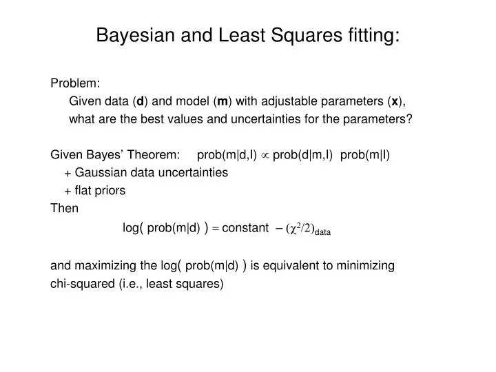
Bayesian and Least Squares fitting:. Problem: Given data ( d ) and model ( m ) with adjustable parameters ( x ), what are the best values and uncertainties for the parameters? Given Bayes’ Theorem: prob(m|d,I) µ prob(d|m,I) prob(m|I) + Gaussian data uncertainties

E N D
Bayesian and Least Squares fitting: Problem: Given data (d) and model (m) with adjustable parameters (x), what are the best values and uncertainties for the parameters? Given Bayes’ Theorem: prob(m|d,I) µ prob(d|m,I) prob(m|I) + Gaussian data uncertainties + flat priors Then log( prob(m|d) )= constant – (c2/2)data and maximizing the log( prob(m|d) ) is equivalent to minimizing chi-squared (i.e., least squares)
M r P Dx M = N and xfitted = x|0 + Dx
Weighted least-squares: Least squares equations: r = PDx , where Pij = ∂mi/∂xj Each datum equation: ri = Sj ( Pij Dxj ) Divide both sides of each equation by datum uncertainty, si , i.e., ri ri / si and Pij Pij / si for each j gives variance-weighted solution.
Including priors in least-squares: Least squares equations: r = d – m = PDx , where Pij = ∂mi/∂xj Each data equation: ri = Sj ( Pij Dxj ) The weighted data (residuals) need not be homogenous: r = ( d – m ) /s can be composed of N “normal” data and some “prior-like data”. Possible prior-like datum: xk = vk ± sk (for kth parameter) Then rN+1 = ( vk - xk ) / sk and PN+1,j = 1/sk for j =k 0 for j ≠ k
Non-linear models Least squares equations: r = PDx, where Pij = ∂mi/∂xj has solution: Dx = (PTP)-1 PTr • If the partial derivatives of the model are independent of the parameters, then the first-order Taylor expansion is exact and applying the parameter corrections, Dx, gives the final answer. Example linear problem: m = x1 + x2 t + x3 t2 • If not, you have a non-linear problem and the 2nd and higher order terms in the Taylor expansion can be important until Dx0; so iteration is required. Example non-linear problem: m = sin(2px1t)
How to calculate partial derivatives (Pij ): • Analytic formulae • (If the model can be expressed analytically) • Numerical evaluations: “wiggle” parameters one at a time: xw = xexcept for jth parameter xjw = xj + dx Partial derivative of the ith datum for parameter j: Pij = ( mi(xw) - mi(x) ) / ( xjw – xj ) NB: choose dx small enough to avoid 2nd order errors, but large enough to avoid numerical inaccuracies. Always use 64-bit computations!
Can do very complicated modeling: Example problem: model pulsating photosphere for Mira variables (see Reid & Goldston 2002, ApJ, 568, 931) Data: Observed flux, S(t,l), at radio, IR and optical wavelengths Model: Assume power-law temperature, T(r,t), and density, r(r,t); calculate opacity sources (ionization equilibrium, H2 formation, …); numerically integrate radiative transfer along ray-paths through atmosphere for many impact parameters and wavelengths; parameters include T0 and r0 at radius r0 Even though model is complicated and not analytic, one can easily calculate partials numerically and solve for best parameter values.
Modeling Mira Variables: Radio: H- free-free opacity at ~2R* IR: seeing pulsating stellar surface Visual:Dmv ~ 8 mag ~ factor of 1000; variable formation of TiO clouds at ~2R* with top T ~ 1400 K
Iteration and parameter adjustment: Least squares equations: r = PDx, where Pij = ∂mi/∂xj has solution: Dx = (PTP)-1 PTr • It is often better to make parameter adjustments slowly, so for the k+1 iteration, set x|k+1= x|k + d*DxIk where 0 < d < 1 • NB: this is equivalent to scaling partial derivatives by d. So, if one iterates enough, one only needs to get the sign of the partial derivatives correct !
Evaluating Fits: Least squares equations: r = PDx, where Pij = ∂mi/∂xj has solution: Dx = (PTP)-1 PTr Always carefully examine final residuals (r) Plot them Look for >3s values Look for non-random behavior Always look at parameter correlations correlation coefficient: rjk = Djk / sqrt( Djj Dkk ) where D = (PTP)-1
sp = 1 / sqrt( S cos2 wt ) • N = 5 • sp = 1 / sqrt( 2 ) = 0.7 • N = 5 • sp = 1 / sqrt( 3 ) = 0.6 • N = 4 • sp = 1 / sqrt( 4 ) = 0.5
Bayesian vs Least Squares Fitting: Least Squares fitting: Seeks the best parameter values and their uncertainties Bayesian fitting: Seeks the posteriori probability distribution for parameters
Bayesian Fitting: Bayesian: what is posterior probability distribution for parameters? Answer, evaluate prob(m|d,I) µ prob(d|m,I) prob(m|I) If data and parameter priors have Gaussian distributions, log( prob(m|d) ) = constant – (c2/2)data – (c2/2)param_priors “Simply” evaluate for all (reasonable) parameter values. But this can be computationally challenging: eg, a modest problem with only 10 parameters, evaluated on a coarse grid of 100 values each, requires 1020 model calculations!
Markov chain Monte Carlo (McMC) methods: Instead of complete exploration of parameter space, avoid regions with low probability and wander about quasi-randomly over high probability regions: “Monte Carlo” random trials (like roulette wheel in Monte Carlo casinos) “Markov chain” (k+1)th trial parameter values are “close to” kth values
McMC using Metropolis-Hastings (M-H) algorithm: • Given kth model (ie, values for all parameters in the model), generate (k+1)th model by small random changes: xj|k+1 = xj|k + a g sj • a is an “acceptance fraction” parameter, • g is a Gaussian random number (mean=0, standard deviation=1), • sj is the width of the posteriori probability distribution of parameter xj • Evaluate the probability ratio: R = prob(m|d)|k+1 / prob(m|d)|k • Draw a random number, U, uniformly distributed from 01 • If R > U, “accept” and store the (k+1)th parameter values, else “replace” the (k+1)th values with a copy the kth values and store them (NB: this yields many duplicate models) Stored parameter values from the M-H algorithm give the posteriori probability distribution of the parameters !
Metropolis-Hastings (M-H) details: M-H McMC parameter adjustments: xj|k+1 = xj|k + a g sj a determines the “acceptance fraction” (start near 1/√N), g is a Gaussian random number (mean=0, standard deviation=1), sj is the “sigma” of the posteriori probability distribution of xj • The M-H “acceptance fraction” should be about 23% for problems with many parameters and about 50% for few parameters; iteratively adjust a to achieve this; decreasing a, increases acceptance rate • Since one doesn’t know the parameter posteriori uncertainties, sj,at the start, one needs to do trial solutions and iteratively adjust. • When exploring the PDF of the parameters with the M-H algorithm, one should start with near-optimum parameter values, so discard early “burn-in” trials.
M-H McMC flow: Enter data (d) and initial guesses for parameters (x, sprior, sposteriori) Start “burn-in” & “acceptance-fraction” adjustment loops (eg, ~10 loops) start a McMC loop (with eg, ~105 trials) make new model: xj|k+1 = xj|k + a g sjposteriori calculate (k+1)th log( prob(m|d) ) µ (c2/2)data + (c2/2)param_priors calculate Metropolis ratio: R = exp( log(probk+1) – log(probk) ) if R > Uk+1 accept and store model < Uk+1 replace with kth model and store end McMC loop estimate & update sposteriori and adjust a for desired acceptance fraction End “burn-in” loops Start “real” McMC exploration with latest parameter values and using final sposteriori and a to determine parameter step sizes. Use a large number of trials (eg, ~106)
Estimation of sposteriori : Make histogram of trial parameter values (must cover full range) Start bin loop check cumulative # crossing “-1s” check cumulative # crossing “+1s” End bin loop Estimates of (Gaussian) sposteriori : • ≈ 0.50 | p_val(+1s) – p_val(-1s) | • ≈ 0.25 | p_val(+2s) – p_val(-2s) | Relatively robust to non-Gaussian pdfs
Adjusting Acceptance Rate Parameter (a): Metropolis trial acceptance rule for (k+1)th trial model: if R > Uk+1 accept and store model < Uk+1 replace with kth model and store For nth set of M-H McMC trials, count cumulative number of accepted (Na) and replaced (Nr) models. Acceptance rate: A = Na / (Na + Nr) For (n+1)th set of trials, set an+1 = (An / Adesired) an
“Non-least-squares” Bayesian fitting: Sivia gives 2 examples where the data uncertainties are not known Gaussians; hence least squares is non-optimal: 1) prob(s÷ s0) = s0 / s2 (for s ≥ s0; 0 otherwise) where s is the error on a datum, which typically is close to s0 (the minimum error), but can occasionally be much larger. 2) prob(s÷ s0,b,g) = b d(s – gs0) + (1-b) d( s – s0) • where b is the fraction of “bad” data whose uncertainties are gso
“Error tolerant” Bayesian fitting: Sivia’s “conservative formulation”: data uncertainties are given by prob(s÷ s0) = s0 / s2 (for s ≥ s0; 0 otherwise) where s is the error on a datum, which typically is close to s0 (the minimum error), but can occasionally be much larger. Marginalizing over s gives prob(d|m,s0) = ∫prob(d |m,s) prob(s÷s0) ds • =∫ (1/s√2p) exp[(d-m)2/2s2] (s0/s2)ds • = (1/s0√2p) ((1 – exp(-R2/2) ) / R2) where R = (d-m)/s0 Thus, one maximizes ∑i log((1 – exp(-R2/2) ) / R2) , instead of minimizing c2/2 = ∑i log(exp(-R2/2) )= ∑i -R2/2
Data PDFs: • Gaussian pdf has sharper peak, giving more accurate parameter estimates (provided all data are good). • Error tolerant pdf doesn’t have a large penalty for a wild point, so it will not “care much” about some wild data.
Error tolerant fitting example: Goal: to determine motion of 100’s of maser spots Data: maps (positions) at 12 epochs Method: find all spots at nearly the same position over all epochs; then fit for linear motion Problem: some “extra” spots appear near those selected to fit (eg, R>10). Too much data to plot, examine and excise by hand.
Error tolerant fitting example: Error tolerant fitting output with no “human intervention”
The “good-and-bad” data Bayesian fitting: Box & Tiao’s (1968) data uncertainties come in two “flavors”, given by prob(s÷ s0,b,g) = b d(s – gs0) + (1-b) d( s – s0) • where b is the fraction of “bad” data ( 0 ≤ b << 1 ), • whose uncertainties are g so ( g >> 1 ) Marginalizing over s for Gaussian errorsgives prob(d|m,s0b,g) = ∫prob(d |m,s,b,g) prob(s÷s0,g,b,g) ds • = (1/s0√2p) ( (b/g) exp(-R2/2g2) + (1-b) exp(-R2/2) ) where R = (d-m)/s0 Thus, one maximizes constant + ∑i log((b/g) exp(-R2/2g2) + (1-b) exp(-R2/2) ) , which for no bad data (b = 0) recovers least squares. But one must estimate 2 extra parameters: b and g
Estimation of parameter PDFs: Bayesian fitting result: histogram of M-H trial parameter values (PDF) This “integrates” over all values of all other parameters and is the parameter estimate “marginalized” over all other parameters. Parameter correlations: e.g, plot all trial values of xi versus xj