Download
1 / 41
410 likes | 559 Views
Discovering Interesting Regions in Spatial Data Sets. Christoph F. Eick Department of Computer Science, University of Houston Motivation: Examples of Region Discovery Region Discovery Framework A Fitness For Hotspot Discovery Other Fitness Functions

E N D
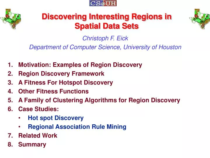
Discovering Interesting Regions inSpatial Data Sets Christoph F. Eick Department of Computer Science, University of Houston Motivation: Examples of Region Discovery Region Discovery Framework A Fitness For Hotspot Discovery Other Fitness Functions A Family of Clustering Algorithms for Region Discovery Case Studies: Hot spot Discovery Regional Association Rule Mining Related Work Summary
Other Contributors to the Work Presented Today Region Discovery Framework • Banafsheh Vaezian (Master student, Department of Computer Science) • Dan Jiang (Master student, Department of Computer Science) Clustering Algorithms for Region Discovery • Jing Wang (Master student, Department of Computer Science) • Wei Ding (PhD student, Department of Computer Science) • Ji Yeon Choo (Master student, Department of Computer Science) • Rachsuda Jiamthapthaksin (PhD student, Department of Computer Science) Regional Association Rule Mining • Wei Ding (PhD student, Department of Computer Science) • Xiaojing Yuan (Faculty Member, College of Technology, UH) Regional Co-location Mining and Spatial Data Mining in General • Spatial Database and Data Mining Group (Shashi Shekhar, UMN) Software Platform and Software Design • Abraham Bagherjeiran (PhD student, Department of Computer Science) Other • Ricardo Vilalta (Faculty Member, Department of Computer Science, UH) • Shahab Khan (Faculty Member, Department of Geosciences, UH)
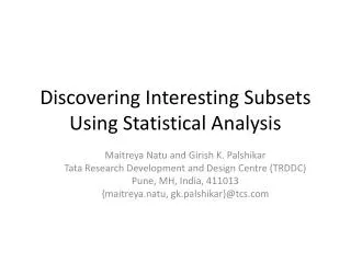
1. Motivation: Examples of Region Discovery Application 1: Hot-spot Discovery [EVDW06] Application 2: Find Interesting Regions with respect to a Continuous Variable Application 3: Find “representative” regions (Sampling) Application 4: Regional Co-location Mining Application 5: Regional Association Rule Mining [DEWY06] Application 6: Regional Association Rule Scoping [EDWYK06] b=1.01 RD-Algorithm b=1.04 Wells in Texas: Green: safe well with respect to arsenic Red: unsafe well
2. Region Discovery Framework • We assume we have spatial or spatio-temporal datasets that have the following structure: (x,y,[z],[t];<non-spatial attributes>) e.g. (longitude, lattitude, class_variable) or (longitude, lattitude, continous_variable) • Clustering occurs in the (x,y,[z],[t])-space; regions are found in this space. • The non-spatial attributes are used by the fitness function but neither in distance computations nor by the clustering algorithm itself. • For the remainder of the talk, we view region discovery as a clustering task and assume that regions and clusters are the same
Region Discovery Framework Continued The algorithms we currently investigate solve the following problem: Given: A dataset O with a schema R A distance function d defined on instances of R A fitness function q(X) that evaluates clustering X={c1,…,ck} as follows: q(X)= cXreward(c)=cXinterestingness(c)*size(c) with b>1 Objective: Find c1,…,ck O such that: • cicj= if ij • X={c1,…,ck} maximizes q(X) • All cluster ciX are contiguous (each pair of objects belonging to ci has to be delaunay-connected with respect to ci and to d) • c1,…,ck O • c1,…,ck are usually ranked based on the reward each cluster receives, and low reward clusters are frequently not reported
Challenges for Region Discovery • Recall and precision with respect to the discovered regions should be high • Definition of measures of interestingness and of corresponding parameterized reward-based fitness functions that capture “what domain experts find interesting in spatial datasets” • Detection of regions at different levels of granularities (from very local to almost global patterns) • Detection of regions of arbitrary shapes • Necessity to cope with very large datasets • Regions should be properly ranked by relevance (reward) • Design and implementation of clustering algorithms that are suitable to address challenges 1, 3, 4, 5 and 6.
3. Fitness Function for Hot Spot Discovery Class of Interest: Unsafe_Well Prior Probability: 20% γ1 = 0.5, γ2 = 1.5; R+ = 1, R-= 1; β = 1.1, =1. 10% 30%
4. Fitness Functions for Other Region Discovery Tasks 4.1 Creating Contour Maps for Water Temperature (Temp) Fig. 1: Sea Surface Temperature on July 7 2002 Var=2.2 Reward: 48,5 Rank: 3 Mean=11.2 A single region and its summary Examples in the data set WT have the form: (x,y,temp); var(c,temp) denotes the variance of variable temp in region c interestingness(c)= IF var(c,temp)>var(WT,temp) THEN 0 ELSE min(1, log20(var(WT,temp)/var(c,temp))) with being a parameter (with default 1) Basically, regions receive rewards if their variance is lower than the variance of the variable temparature for the whole data set, and regions whose variance is at least 20 times less receive the maximum reward of 1.
4.2 Regional Co-location Mining R1 R2 Regional Co-location R3 R4 Task: Find Co-location patterns for the following data-set. Global Co-location: and are co-located in the whole dataset
A Reward Function for Binary Co-location Task: Find regions in which the density of 2 or more classes is elevated. In general, multipliers lC are computed for every region r, indicating how much the density of instances of class C is elevated in region r compared to C’s density in the whole space, and the interestness of a region with respect to two classes C1 and C2 is assessed proportional to the product lC1*lC2 Example: Binary Co-Location Reward Framework; lC(r)=p(C,r)/prior(C) C1,C2 = 1/((prior(C1)+prior(C2)) “maximum multiplier” kC1,C2(r) = IF lC1(r)<1 or lC2(r )<1 THEN 0 ELSE sqrt((lC1(r)–1)*(lC2(r)–1))/(C1,C2 –1) interestingness(r)= maxC1,C2;C1C2 (kC1,C2(c))
How to Apply the Suggested Methodology • With the assistance of domain experts determine structure of dataset to be used. • Acquire measure of interestingness for the problem of hand (this was purity, variance, probability elevation of two or more classes in the examples discussed before) • Convert measure of interestingness into a reward-based fitness function. The designed fitness function should assign a reward of 0 to “boring” regions. It is also a good idea to normalize rewards by limiting the maximum reward to 1. • After the region discovery algorithm has been run, rank and visualize the top k regions with respect to rewards obtained (interestingness(c)*size(c)), and their properties which are usually task specific.
5. A Family of Clustering Algorithms for Region Discovery • Supervised Partitioning Around Medoids (SPAM). • Single Representative Insertion/Deletion Steepest Decent Hill Climbing with Randomized Restart (SRIDHCR). • Supervised Clustering using Evolutionary Computing (SCEC) • Agglomerative Hierarchical Supervised Clustering (SCAH) • Hierarchical Grid-based Supervised Clustering (SCHG) • Supervised Clustering using Multi-Resolution Grids (SCMRG) • Representative-based Clustering with Gabriel Graph Based Post-processing (SCEC+PGPP / SRIDHCR+PGPP) • Supervised Clustering using Density Estimation Techniques (SCDE) Remark: For a more details: SCEC, SPAM, and SRIDHCR[EZZ04, ZEZ06]; [SCAH] and SCHG [EVJW04], SCMRG [EDWYK06],…+PGPP[CJCCE06]
SCAH (Agglomerative Hierarchical) Inputs: A dataset O={o1,...,on} A distance Matrix D = {d(oi,oj) | oi,oj O }, Output: Clustering X={c1,…,ck} Algorithm: 1) Initialize: Create single object clusters: ci = {oi}, 1≤ i ≤ n; Compute merge candidates based on “nearest clusters” 2) DO FOREVER a) Find the pair (ci, cj) of merge candidates that improves q(X) the most b) If no such pair exist terminate, returning X={c1,…,ck} c) Delete the two clusters ci and cjfrom X and add the cluster ci cj to X d) Update inter-cluster distances incrementally e) Update merge candidates based on inter-cluster distances
SCHG (Hierarchical Grid-based) Remark: Same as SCAH, but uses grid cells as initial clusters Inputs: A dataset O={o1,...,on} A grid structure G Output: Clustering X={c1,…,ck} Algorithm: 1) Initialize: Create clusters making each single non-empty grid cell a cluster Compute merge candidates (all pairs of neighboring grid cells) 2) DO FOREVER a) Find the pair (ci, cj) of merge candidates that improves q(X) the most b) If no such pair exist terminate, returning X={c1,…,ck} c) Delete the two clusters ci and cjfrom X and add the cluster c’=ci cj to X d) Update merge candidates: cX (MC(c’,c) MC(c, ci) MC(c, cj ))
Ideas SCMRG (Divisive, Multi-Resolution Grids) Cell Processing Strategy 1. If a cell receives a reward that is larger than the sum of its rewards its ancestors: return that cell. 2. If a cell and its ancestor do not receive any reward: prune 3. Otherwise, process the children of the cell (drill down)
Representative-based Clustering 2 Attribute1 1 3 Attribute2 4 Objective: Find a set of objects OR such that the clustering X obtained by using the objects in OR as representatives minimizes q(X). Properties: Cluster shapes are convex polygons Popular Algorithms: K-means. K-medoids
Proximity Graph-Based Post-Processing[CJCCE06] Before After Idea: Clusters with arbitrary shapes are approximated using unions of small convex polygons (that have been obtained by running a representative-based clustering algorithm, such as k-medoids)
Pseudo Code PGPP 1. Run a representative-based clustering algorithm to create a large number of clusters. 2. Read the representatives of the obtained clusters. 3. Create a merge candidate relation using proximity graphs. 4. WHILE there are merge-candidates (Ci ,Cj) left whose merging enhances q(X) BEGIN Merge the pair of merge-candidates (Ci,Cj), that enhances fitness function q the most, into a new cluster C’=CiCj Update Merge-Candidates: C (Merge-Candidate(C’,C) Merge-Candidate(Ci,C) Merge-Candidate(Cj,C)) END 5. RETURN the best clustering X found.
Comparison of PGPP with K-means (a) K-means (b) Post-processing with q1(X) (c) Post-processing with q2(X)
6a. Applications to Hotspot Discovery Volcano Earthquake
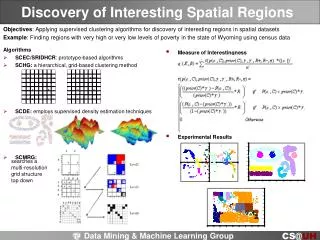
Experimental Evaluation • SCAH outperforms SCHG and SCMRG when the penalty for the number of clusters is very low (b=1.01, =6). However, when SCAH runs out of pure clusters to merge, it has the tendency to terminate prematurely; therefore, it does quite poorly when the objective is obtain large clusters (b=3, =1). • SCHG outperforms SCMRG and SCAH for b=3, =1. • SCMRG obtains better clusters than SCAH for the Volcano dataset for b=1.01, =6, which can be attributed to the fact that SCMRG uses grid cells with different sizes. • Avg. wall clocktime for smaller datasets SCAH:SCMRG/SCHG: 13:1/52:1 • SCAH is not suitable to cope with dataset sizes of 10000 and more, mainly because of the large number of distance computations, large numbers of clusters, and merge steps needed. • The quality of clustering of SCMRG is strongly dependent on initial cluster sizes and on the look ahead depth.
Problems with SCAH Too restrictive definition of merge candidates: XXXOOO OOOXXX No look ahead: Non-contiguous clusters:
6.b: Regional Association Mining Example of an Association Rule: • IF the well’s water is used by humans • and the well’s nitrate level is above 28.5 • and the well’s fluoride level is between 0.005 and 0.195 • THENthe well has dangerous levels of arsenic (support=0.5%, confidence=87%).
Why Regional Knowledge Important in Spatial Data Mining? • A special challenge in spatial data mining is that information is usually not uniformly distributed in spatial datasets. • It has been pointed out in the literature that “whole map statistics are seldom useful”, that “most relationships in spatial data sets are geographically regional, rather than global”, and that “there is no average place on the Earth’s surface” [Goodchild03, Openshaw99]. • Therefore, it is not surprising that domain experts are mostly interested in discovering hidden patterns at a regional scale rather than a global scale.
Regional Association Rule Mining • Most data mining techniques are ill-prepared for discovering regional knowledge. For example, in traditional association rule mining, regional patterns frequently fail to be discovered due to insufficient global confidence and/or support. • This raises the questions on how to identify interesting regions algorithmically, and how to measure the scope of a regional association rule
Regional Association Rule Mining and Scoping • Steps Regional Association Rule Mining • Find regions • Mine regional association rules [DEWY06] • Find the scope of discovered regional association rules[SDM06]
Association Rule Scope Discovery Framework Let a be an association rule, r be a region, conf(a,r) denotes the confidence of a in region r, and sup(a,r) denotes the support of a in r. Goal: Find all regions for which an associate rule a satisfies its minimum support and confidence threshold; regions in which a’s confidence and support are significantly higher than the min-support and min-conf thresholds receive higher rewards. Association Rule Scope Discovery Methodology: For each rule a that was discovered for region r’, we run our region discovery algorithm that defines the interestingness of a region ri with respect to an association rule a as follows: Remarks: • Typically d1=d2=0.9; =2 (confidence increase is more important than support increase) • Obviously the region r’ from which rule a originated or some variation of it should be “rediscovered” when determining the scope of a.
Region vs. Scope • Scope of an association rule indicates how regional or global a local pattern is. • The region, where an association rule is originated, is a subset of the scope where the association rule holds.
Fine Tuning Confidence and Support • We can fine tune the measure of interestingness for association rule scoping by changing the minimum confidence and support thresholds.
7. Related Work • In contrast to most work in spatial data mining, our work centers on creating regional knowledge and not global knowledge. • A lot of work in spatial data mining centers on partioning a spatial dataset into “transactions” so that apriori-style algorithms can be used. We claim that our work can contribute to “finding such transactions” [DEWY06]. • Our work related to hotspot discovery has similarity to work in supervised clustering/semi-supervised clustering in that it uses class labels in evaluating clusters. Moreover, the goals of the algorithms presented are similar to hotspot discovery algorithms, a task that does not receive a lot of attention in spatial data mining, but more attention by scientists in earth sciences and related disciplines.
8. Summary • A framework for region discovery that relies on additive, reward-based fitness functions and views region discovery as a clustering problem has been introduced. • Families of clustering algorithms and measures of interested are provided that form the core of the framework. • Evidence concerning the usefulness of the framework for regional association rule mining amd hotspot discovery has been presented. • The special challenges in designing clustering algorithms for region discovery have been identified. • The ultimate vision of this research is the development of region discovery engines that assist earth scientists in finding interesting regions in spatial datasets.
The Ultimate Vision of the Presented Research DomainExpert Spatial Databases Family of Measures of interestingness Measure ofInterestingness Acquisition Tool Database Integration Tool Fitness Function Data Set Family of Clustering Algorithms Region DiscoveryDisplay Ranked Set of Interesting Regions and their Properties Visualization Tools Architecture Region Discovery Engine
Why should people use Region Discovery Engines (RDE)? RDE: finds sub-regions with special characteristics in large spatial datasets and presents findings in an understandable form. This is important for: • Focused summarization • Find interesting subsets in spatial datasets for further studies • Identify regions with unexpected patterns; because they are unexpected they deviate from global patterns; therefore, their regional characteristics are frequently important for domain experts • Without powerful region discovery algorithms, finding regional patters tends to be haphazard, and only leads to discoveries if ad-hoc region boundaries have enough resemblance with the true decision boundary • Exploratory data analysis for a mostly unknown dataset • Co-location statistics frequently blurred when arbitrary region definitions are used, hiding the true relationship of two co-occurring phenomena that become invisible by taking averages over regions in which a strong relationship is watered down, by including objects that do not contribute to the relationship (example: High crime-rates along the major rivers in Texas) • Data set reduction; focused sampling
Additional Transparencies Additional Transparencies On Region Discovery Not Used in Lecture
Experimental Results Volcano for b=1.01, =6 SCAH SCHG SCMRG
Using Gabriel Graphs to Determine Neighboring Clusters • VolcanoK = 100 Gabriel Graphs: (Ci, Cj) having an edge implies that Ci and Cj are neighboring
Datasets Used • Obtained from Geosciences Department in University of Houston. • The Earthquake dataset contains all earthquake data worldwide done by the United States Geological Survey (USGS) National Earthquake Information Center (NEIC). • The modified Earthquake dataset contains the longitude, latitude and a class variable that indicates the depth of the earthquake, 0(shallow), 1(medium) and 2(deep).
Datasets Used • Wyoming datasets were created from U.S. Census 2000 data. • The Wyoming Modified Poverty Status in 1999 is a modified version of the original dataset, Wyoming Poverty Status. • The Wyoming Poverty Datasets were created using county statistics. For each county, random population coordinates were generated using the complete spatial randomness (CSR) functions in S-PLUS. • Then, the background information was attached to each individual county based on the county’s distribution for the class of interest. Finally, all counties were merged into a single dataset that describes the whole state.
Datasets Used • Obtained from Geosciences Department in University of Houston. • The Volcano dataset contains basic geographic and geologic information for volcanoes thought to be active in the last 10,000 years • The original data include a unique volcano number, volcano name, location, latitude and longitude, summit elevation, volcano type, status and the time range of the last recorded eruption. • The Subset of the volcano dataset used in this thesis contains longitude, latitude and a class variable that indicates if a volcano is non –violent (blue) or violent (red).