Download

1 / 30
330 likes | 522 Views
Two-Way ANOVA. Lab 5 instruction. ANOVA: analysis of variance. a collection of statistical methods to compare several groups according to their means on a quantitative response variable Two-Way ANOVA two factors are used consider “main effect” and “interaction effect”. Example.

E N D
Two-Way ANOVA Lab 5 instruction
ANOVA: analysis of variance • a collection of statistical methods to compare several groups according to their means on a quantitative response variable • Two-Way ANOVA two factors are used consider “main effect” and “interaction effect”
Example • Response: Blood Alcohol Content (BAC) • Factors: • Gender(GEN) • Alcohol Consumption (ALC) • Factor levels: • GEN: 1=Male; 0=Female • ALC: 1=1 drink; 2=2 drinks; 4=4 drinks • Main effect of GEN, main effect of ALC, and their interaction
Explore the difference in average response across both factors. • Table of marginal means (contingency table) • In SPSS: Analyze Compare Means Means /Or General linear models descriptive stat
e.g. Table of marginal means (contingency table) • Response: in Dependent list • Factors: in independent list of two seperate layers
e.g. Table of marginal means (contingency table) • Interpret
Explore the difference in average response across both factors. • Plots of marginal means (profile plot) • In SPSS: Graphs legacy dialogs Line multiple /Or GLM univariate (plots)
e.g. Plot of marginal means (profile plot) • Profile plot with lines representing gender
e.g. Plot of marginal means (profile plot) • Interpretation: • 6 points • Effect of gender • Effect of drink consumption • Interaction (parallel or crossed)
Explore the difference in average response across both factors. • Clustered boxplot • In SPSS: Graphs legacy dialogs Boxplot Clustered
e.g. Clustered boxplot • Clustered boxplot with clusters defined by gender
General Linear Model (GLM)-Assumptions • Independent samples • Normality: • Boxplot • QQ plot • Equal standard deviation (variance): • Boxplot • Summary statistics (rule of thumb: the ratio of the largest s.d. over the smallest s.d. is less than 2)
General Linear Model (GLM) • Univariate GLM is the general linear model now often used to implement such essential statistical procedures as regression and ANOVA. In particular, the procedure can be used to carry out two-way analysis of variance. • Procedure: Analyze General Linear Model Univariate (defaulted: model with Interactions)
GLM: Non-additive model output • In columns “SS” and “df” • Corrected total = corrected model + error • Corrected model=GEN + ALC + GEN*ALC • The column “F” contains the value of the f statistic for each effect. The value of F is computed as follows:
GLM: Non-additive model output Hypothesis test : no interaction between GEN and ALC
Equivalent to the regression models: Since the interaction term is not significant, we tend to modify the model. the model without the interaction term: additive model
GLM - Options • Model: define the model, Include intercept or not • Contrasts: The linear combination of the level means • Profile Plots: the plot of estimated means • Post Hoc • Save • Options
GLM - Options • Profile Plots: different from the one obtained with line chart • This plots estimated means form the model
Equivalent regression models and tests • Define dummy variables • Write down estimated model equation • Use extra-sum-of-squares F-test for testing interaction term • Interpret meaning of estimated coefficient, t-test on coefficients and their 95% CI
Equivalent regression models and tests • estimated regression model with interaction term (full non-additive model)
Equivalent regression models and tests • estimated regression model with NO interaction term (additive model)
Equivalent regression models and tests • Construct extra-of-sum F-test use the above two ANOVA tables, • In the regression model with NO interaction term, interpret meaning of , and its CI. • Is “GEN” effective in predicting BAC? (t-test on )
Note on Q3 (b) • Linear combination of mean difference in BAC for male V.S. female • Substitute ’s by corresponding ’s
Note on Q3 (c) and Q7 (c) • Rate of increase in mean BAC for an increase in drinks consumption • Thus, in Q3 (c) • rate (1to2) = , rate (2to4) = • In Q7 (c) • rate (1to2) = , rate (2to4) =