n (0,1)

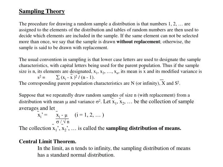
1. Sampling TheoryThe procedure for drawing a random sample a distribution is that numbers 1, 2, … are assigned to the elements of the distribution and tables of random numbers are then used to decide which elements are included in the sample. If the same element can not be selected more than once, we say that the sample is drawn without replacement; otherwise, the sample is said to be drawn with replacement.The usual convention in sampling is that lower case letters are used to designate the sample characteristics, with capital letters being used for the parent population. Thus if the sample size is n, its elements are designated, x1, x2, …, xn, its mean is x and its modified variance is s2 = å (xi - x )2 / (n - 1).The corresponding parent population characteristics are N (or infinity), X and S2.Suppose that we repeatedly draw random samples of size n (with replacement) from a distribution with mean m and variance s2. Let x1, x2, … be the collection of sample averages and let xi’ = xi - m(i = 1, 2, … )s / Ö nThe collection x1’, x2’, … is called the sampling distribution of means.Central Limit Theorem.In the limit, as n tends to infinity,the sampling distribution of means has a standard normal distribution.

2. Attribute and Proportionate SamplingIf the sample elements are a measurement of some characteristic, we are said to have attribute sampling. On the other hand if all the sample elements are 1 or 0 (success/failure,agree/ no-not-agree), we have proportionate sampling. For proportionate sampling, the sample average x and the sample proportion p are synonymous, just as are the mean m and proportion P for the parent population. From our results on the binomial distribution, the sample variance is p (1 - p) and the variance of the parent distribution is P (1 - P).We can generalise the concept of the sampling distribution of means to get the sampling distribution of any statistic. We say that a sample characteristic is an unbiased estimator of the parent population characteristic, is the mean of the corresponding sampling distribution is equal to the parent characteristic.Lemma. The sample average (proportion ) is an unbiased estimator of the parent average (proportion): E [ x] = m; E [p] = P.The quantity Ö ( N - n) / ( N - 1) is called the finite population correction (fpc). If the parent population is infinite or we have sampling with replacement the fpc = 1.Lemma. E [s] = S * fpc.

3. Confidence IntervalsFrom the statistical tables for a standard normal distribution, we note that Area Under From To Density Function 0.90 -1.64 1.64 0.95 -1.96 1.96 0.99 -2.58 2.58 From the central limit theorem, if x and s2 are the mean and variance of a random sample of size n (with n greater than 25) drawn from a large parent population, then we can make the following statement about the unknown parent mean m Prob { -1.64 £ x - m£ 1.64) » 0.90s / Ö ni.e. Prob { x - 1.64 s / Ö n £ m£ x + 1.64 s / Ö n } » 0.90The range x + 1.64 s / Ö n is called a 90% confidence interval for the population mean m.Example [ Attribute Sampling]A random sample of size 25 has x = 15 and s = 2. Then a 95% confidence interval for m is 15 + 1.96 (2 / 5) (i.e.) 14.22 to 15.78Example [ Proportionate Sampling]A random sample of size n = 1000 has p = 0.40 Þ 1.96 Ö p (1 - p) / (n) = 0.03.A 95% confidence interval for P is 0.40 + 0.03 (i.e.) 0.37 to 0.43. n (0,1) 0.95 -1.96 0 +1.96

4. Small Sampling TheoryFor reference purposes, it is useful to regard the expression x ± 1.96 s / Ö nas the “default formula” for a confidence interval and to modify it to suit particular circumstances. O If we are dealing with proportionate sampling, the sample proportion is the sample mean and the standard error (s.e.) term s / Ö n simplifies as follows: x -> p and s / Ö n -> Ö p(1 - p) / (n). O A 90% confidence interval will bring about the swap 1.96 -> 1.64. O If the sample size n is less than 25, the normal distribution must be replaced by Student’s t n - 1 distribution. O For sampling without replacement from a finite population, a fpc term must be used.The width of the confidence interval band increases with the confidence level.Example. A random sample of size n = 10, drawn from a large parent population, has a mean x = 12 and a standard deviation s = 2. Then a 99% confidence interval for the parent mean is x ± 3.25 s / Ö n (i.e.) 12 ± 3.25 (2)/3.2 (i.e.) 9.83 to 14.17and a 95% confidence interval for the parent mean is x ± 2.262 s / Ö n (i.e.) 12 ± 2.262 (2)/3.2 (i.e.) 10.492 to 13.508.Note that for n = 1000, 1.96 Ö p (1 - p) / n » 0.03 for values of pbetween 0.3 and 0.7. This gives rise to the statement that public opinion polls have an “inherent error of 3%”. This simplifies calculations in the case of public opinion polls for large political parties.