Download
1 / 83
1.11k likes | 2.76k Views
Flow Over a Cylinder. Flow over a cylinder Finite Element Tutorial By Dr. Essam A. Ibrahim, Tuskegee University, Mechanical Engineering Dept., emeei@tuskegee.edu Copyright 2006 Expected completion time for this tutorial: 45 minutes to 1 hour Companion tutorial for Fluid Mechanics Course

E N D
Flow Over a Cylinder • Flow over a cylinder Finite Element Tutorial • By Dr. Essam A. Ibrahim, Tuskegee University, Mechanical Engineering Dept., emeei@tuskegee.edu Copyright 2006 • Expected completion time for this tutorial: 45 minutes to 1 hour • Companion tutorial for Fluid Mechanics Course • Reference Text: Fluid Mechanics, 5th Edition, by Frank M. White
Table of Contents • Educational Objectives • Problem Description • Introduction to COSMOSFloWorks • Step by Step Process • Viewing the Results of the FE Analysis • Comparison of Analytical to Finite Element Analysis • Conclusion • Acknowledgment
Educational Objectives 1. Be familiar with the basis of FE theory for two-dimensional flow analysis. 2. Understand the fundamentals of external flow over cambered bodies through the use of the COSMOSFloWorks finite element software. 3. Be able to construct a correct solid model using the SolidWorks CAD and perform an accurate finite element analysis using COSMOSFloWorks. 4. Know how to interpret and evaluate finite element solution quality including verifying analytically the drag coefficient of a cylinder immersed in a uniform fluid stream. 5. Learn to apply the appropriate ambient and boundary conditions and decide on the suitable size for the computational domain.
Problem Description • In this tutorial we use COSMOSFloWorks to determine the aerodynamic drag coefficient of a circular cylinder immersed in a uniform fluid stream. The cylinder axis is oriented perpendicular to the stream. • The computations are performed for Reynolds number = 10 and 1,000 where Re = UD/ = UD/, D is the cylinder diameter, U is the velocity of the fluid stream, and , and are the fluid density, dynamic viscosity and kinematic viscosity, respectively.
Problem Description • The aerodynamic drag coefficient for the cylinder is defined as: where FD is the total force in the flow direction (i.e. drag) acting on a cylinder of diameter D and length L. • The Goal of the simulation is to obtain the drag coefficient for a circular cylinder of D = L = 0.1m, placed in air stream at 20 C using COSMOS FloWorks and compare it with experimental data.
Introduction to COSMOSFloWorks Overview • COSMOSFloWorks 2007 Capabilities • Governing Equations of Fluid Motion • COSMOSFloWorks Theoretical Background • Fluid Flow Terminology • Steps to Analysis • COSMOSFloWorks Project • Ambient and Boundary Conditions
Introduction to COSMOSFloWorks Overview • Run, Solve • Solve Command • Monitoring the Solution • FloWorks Results
COSMOSFloWorks 2007 Capabilities • COSMOSFloWorks is based on advanced Computational Fluid Dynamics (CFD) techniques and allows you to analyze a wide range of complex flows with the following characteristics:
COSMOSFloWorks 2007 Capabilities • Two- and Three-Dimensional analyses • External and Internal Flows • Steady-state and Transient flows • Incompressible liquid and Compressible gas flows including subsonic, transonic and supersonic regimes
COSMOSFloWorks 2007 Capabilities • Non-Newtonian liquids*(laminar only) • Compressible liquids* (liquid density is dependent on pressure) • Laminar, turbulent, and transonic flows • Swirling flows and Fans • Multi-species flows • Flows with Heat Transfer within and between fluids and solids (Conjugate Heat Transfer) • *Professional Version only
COSMOSFloWorks 2007 Capabilities • Surface-to-surface radiation* (including solar heating) • Flows with Gravitational effects (also known as buoyancy effects) • Porous media • Fluid flows with liquid droplets or solid particles • Walls with roughness • Tangential motion on walls* (translation and rotation)
Governing Equations of Fluid Motion • COSMOSFloWorks solves the full Navier-Stokes Equations- The equations are supplemented by fluid state equations defining the nature of the fluid, and by empirical laws for dependency of viscosity and thermal conductivity on other flow parameters • Conservation equations are conserved • Conservation of mass (Continuity equation) • Newton’s second law of motion( Momentum Equation) • The First Law of Thermodynamics (Conservation of Energy Equation) • Transport equations are used for turbulent kinetic energy and dissipation rate (k-e model)
COSMOSFloWorks Theoretical Background • COSMOSFloWorks solves the governing equations using the finite volume (FV) method rather than the finite element method • On spatially rectangular computational mesh designed in the Cartesian coordinate system • With the planes orthogonal to its axes and refined locally a the solid/fluid interface. • And, if necessary, additionally in specified fluid regions, at the solid/solid interfaces, and in the fluid region during calculation.
COSMOSFloWorks Theoretical Background • Values of all physical variables are stored at the mesh centers.. • The governing equations are discretized in a conservation form. • The spatial derivatives are approximated with implicit difference operators of second order accuracy.
COSMOSFloWorks Theoretical Background • A laminar/turbulent boundary layer model is used to describe flows in near-wall regions. The model is based on the so-called Modified Wall Functions approach. • This model is employed to characterize laminar and turbulent flows near walls, and to describe transitions from laminar to turbulent flow and vice versa.
COSMOSFloWorks Theoretical Background • Iterative Methods for Nonsymmetrical Problems • To solve the asymmetric systems of linear equations that arise from approximations of momentum, temperature and species equations, preconditioned generalized conjugate gradient method is used. Incomplete LU factorization is used for preconditioning. • Iterative Methods for Symmetric Problems • To solve symmetric algebraic problem for pressure-correction an original double-preconditioned iterative procedure is used. It is based on a specifically developed multigrid method.
Fluid Flow Terminology • COMOSFloWorks always uses absolute pressure • Absolute Pressure- when pressure is given relative to zero pressure (i.e. psia) • Gage Pressure-when pressure is given relative to the atmospheric pressure of the surroundings (i.e. psig) • For example at sea level the absolute pressure would be 14.6959 psia (pounds per square inch absolute, or 0.00 psig (pounds per square inch gage) if the gage were set to sea level pressure.
Fluid Flow Terminology • There are two ways to measure pressure in fluid flow: Static Pressure, P, and Total (Stagnation) Pressure, • Static pressure is the pressure indicated by a measuring device moving with the flow or by a device that introduces no change to the flow. • Total pressure is the pressure measured by bringing the flow to rest isentropically (without loss)
Fluid Flow Terminology • Dynamic pressure • Dynamic pressure can also be defined as the difference between Total pressure and Static pressure • For compressible flow • Using state adiabatic equations and the gas state equation ( ) the relation between static and total pressure can be written.
Steps to Analysis • Create design in SolidWorks • FloWorks can analyze Parts, Assemblies, Subassemblies, Multibodies • Create COSMOSFloWorks Project file • Use FloWorks Wizard to create project file
COSMOSFloWorks Project • A COSMOSFloWorks project contains all the settings and results of a problem. • Each COSMOSFloWorks project is associated with a SolidWorks configuration • By modifying a COSMOSFloWorks project you can analyze flows under various conditions and for modified SolidWorks models • When a basic project has been created, a new COSMOSFloWorks Design Tree tab appears on the right of the right side of the SolidWorks Configuration Manager tab. • You can use the COSMOSFloWorks Design Tree to specify the remaining project data such as boundary conditions, initial conditions, heat sources, material conditions, and goals.
COSMOSFloWorks Project • To create a project, you must define the following: • A project name • A system of units • An analysis type (external or internal) • The type of fluid (gas, incompressible liquid, Non-Newtonian laminar liquid, or compressible liquid)
Overview of SolidWorks Window • Menu bar • Sketch toolbar/Sketch Relations toolbar • Confirmation Corner with sketch indicator • Graphics area • Sketch origin • Reference Triad
COSMOSFloWorks Project • To create a project, you must also define the following (if applicable): • The substances (fluids and solids) • Initial or ambient conditions • The geometry resolution and the results resolution • A wall roughness value • Physical features include heat transfer in solids, high Mach number gas flow effects, gravitational effects, time dependent effects, surface-to-surface radiation and laminar only flow.
COSMOSFloWorks Project • To create a project, you define the following (if applicable): • Default wall conditions, e.g. adiabatic wall, if heat transfer in solids is not considered. • Default outer wall thermal conditions in case of internal analysis with heat transfer, • Default radiation wall conditions in case of surface-to-surface radiation
Wall Boundary Conditions • The default velocity boundary conditions at solid walls corresponds to the no-slip condition (velocity goes to zero at the wall). • The ”Ideal Wall” condition is also available. For example Ideal Walls can be used to model planes of flow symmetry.
COSMOSFloWorks Project • You can create a new COSMOSFloWorks project in three ways: • 1. The Wizard is the most straightforward way to create a COSMOSFloWorks project. It guides you step-by-step through the analysis set-up process. • 2. You can create a COSMOSFloWorks project by using a Template created from a previous COSMOSFloWorks project. Then click Project, NEW and enter the required information. • 3. To analyze different flow or model variations, the most efficient method is to clone (copy) your current project. The new project will have all the settings of the cloned project, including the results settings.
Run , Solve • COSMOSFloWorks discretizes the time –de-pendent Navier-Stokes equations and solves them on the computational mesh. • Under certain conditions, to resolve the solution’s features better, COSMOSFloWorks will automatically refine the computational mesh during the flow calculation. • Since COSMOSFloWorks solves steady-state problems by solving time-dependent equations, COSMOSFloWorks has to decide when a steady-state solution is obtained ( i.e. the solution converges), so that the calculation can be stopped. COSMOSFloWorks offers for you a choice of different conditions to finishing the calculation.
Monitoring the Solution • Goals Tab • Monitor each goal for convergence; it should flatten out • Its good practice to monitor mass balance (SG’s) • You can stop the calculation and view the results to determine if additional iterations are necessary • Preview Tab • Check flow behavior to ensure proper set up • Info Tab • Cell count, CPU time, & No. of Iterations
FloWorks Results • Results Plots (Qualitative) • Vectors, Contours, Isolines • Cut Plots, Surface Plots, Flow Trajectories, Isosurfaces • Processed Results (Quantitative) • X-Y plots (Excel) • Goals (Excel) • Surface Parameters • Point Parameters • Report • Reference Fluid Temperature
Solve Command • To solve your project ,go to the FloWorks command line and click Solve. • You will have one of two methods to solve your project • RUN • BATCH RUN
Using the SolidWorks Interface • Toolbar area • Feature Manager window • Graphical Interface window
Overview of SolidWorks Window • Menu bar • Sketch toolbar/Sketch Relations toolbar • Confirmation Corner with sketch indicator • Graphics area • Sketch origin • Reference Triad
Left Side of SolidWorks Window • Feature Manager icon • Feature Manager design tree • COSMOSWorks icon • COSMOSWorks Manager tree
Toolbars • You can select which toolbars to display under View in the menu heading • Toolbars are moveable to top, and sides of the window • Icon Buttons for frequently used commands
Create a New Part • In SolidWorks main tool bar click File, New.The New Solid Document window appears • The part icon is highlighted • Click OK. The SoliWorks graphical interface window appears.
Sketch Part • In SolidWorks menu tool bar click the Sketch icon • A menu of shapes appears. Select circle
Create a Plane • The Front, Top, and Right planes appear in the graphical interface window • Select the Front plane to start the sketch. The display changes so that the front plane is facing you. A sketch opens on the front plane.
Draw a Circle • Move the pointer in the graphical interface window to the sketch origin and drag the mouse to draw a circle • In the circle command window adjust the circle radius to 50 mm or 5cm. • Accept the new dimensions by clicking the check mark .
Create a Cylinder • In the SolidWorks menu bar click the Feature icon and select Extruded/Boss Base • The circle is extruded into a cylinder. In the Extrude window set the cylinder length to 100 mm or 10 cm • Accept the part by clicking the check mark.
Save Part • The part is displayed as Trimetric view. To change the view to Isometric click the view tab located at the lower left corner of the graphical interface window area and choose Isometric • To save the part, click File, Save as in the SolidWorks menu bar. Save the part in my documents folder under the name cylinder
Importing the Solid Part • Click File, Open, my documents folder opens • Select the file named “cylinder” which contains the part previously created using SolidWorks • The part is imported
Create New Configuration • Click FlowWorks on the main toolbar then click Project, Wizard (The Wizard guides you through the definition of a new project) • Select Create new. In the configuration name type Cylinder_Re_ 10 • Click Next
Select Unit System • In the Unit System dialog box you can select the desired system of units for both input and output (results) • Specify the International System SI by default • Click Next
Specify Analysis Type • In the Analysis Type dialog box select an External type of flow analysis. This dialog box allows you to specify advanced physical features you want to include in the analysis. In this project we will not use any of the advanced physical features • Click Next
Choose Default Fluid • In the Default Fluid dialog box open the Gases folder (by clicking the square to its left) • Double-click the Air item • Click Next
Set Wall Conditions • Since we don’t intend to calculate heat conduction in solids, we keep the default Adiabatic wall setting denoting that all the model walls are heat insulated • We also keep the default 0 micrometer wall roughness • Click Next
Initial and Ambient Conditions • In the Initial and Ambient Conditions dialog box we specify the incoming flow velocity by clicking the Velocity in X direction box • The Dependency button is enabled • Click Dependency. The Dependency dialog box appears
Velocity Calculation Formula • In the Dependency type list select Formula definition • In the Formula box type the formula defining the flow velocity using Reynolds number = 10. Here the kinematic viscosity of air is n=1.51E-5 m2 /sec at a temperature of 293.2 K and the cylinder diameter is 0.1 m. • Click OK you will return to the Initial and Ambient Conditions dialog box.
Results and Geometry resolution • In the Results and Geometry Resolution specify a result resolution level of 7 • Accept the automatically defined minimum gap size and wall thickness • Click Finish. The project is created and the 3D Computational Domain is automatically generated