Download
1 / 28
280 likes | 529 Views
WISP Localization. Jonathan Huang and Ali Rahimi. The Localization Problem. Track the 3D position and rotation of a WISP based on harvested signal strengths. WISP Power Harvester. Chair. This is difficult. The mapping from positions to voltages is environment specific

E N D
WISP Localization Jonathan Huang and Ali Rahimi
The Localization Problem Track the 3D position and rotation of a WISP based on harvested signal strengths WISP Power Harvester
This is difficult • The mapping from positions to voltages is environment specific • Most environments are too complex to be analytically modeled • Voltage measurements are noisy
Approach • Ultimate goal: learn the mapping from positions to voltages while tracking • But for now: learn the mapping from ground truth obtain by camera system
Current Approach • Collect ground truth for training and evaluation • Learn the function which maps positions to voltage readings • Use dynamics to track tags
Processing the Voltage Readings Raw Signal (3 Antennas)
Processing the Voltage Readings • The Alien Reader cycles through each antenna. Each cycle begins with a spike and ends with a long rest • The received signal is actually a somewhat corrupted version of this: (Zoomed In)
Processing the Voltage Readings HMM signal model States: long break, start spike, ant1, ant2, ant3, short break Observations: >thresh, <thresh Parse using Viterbi to separate signal from spurious spikes, and to get antenna id.
Processing the Voltage Readings Raw Signal (with errors shown) The most-likely parse as determined by Viterbi
Processing the Voltage Readings For each antenna, we average all of the readings in one frame to obtain the final signal 20 seconds 4 seconds
Visual Localization • Setup: Groundtruthing cameras Testing and data collection setup RFID antenna Lights to simplify camera-based tracking RFID antenna
Calibrating the Camera Setup Input Images with corner detections Recovered Camera Pose
Input Thresholded Background Subtraction Thresholded Brightness Connected Components Labeling Estimate the mean of the largest two components Output
Vision Results • Performance • 15 fps, processing two time-synced PtGrey Dragonfly2 cameras • Limitations • Algorithm sensitive to lighting conditions, random movements • Works well when lighting is constant and scene is static (except for the lights) • The known distance between the lights provides a sanity check and adds robustness
Current Approach • Collect ground truth for training and evaluation • Learn the function which maps positions to voltage readings • Use dynamics to track tags
One Dimensional Localization • Data Collection • We waved a WISP in (roughly) a straight line between two antennas • Learning • We regressed positions against two voltage readings using a Gaussian Process model
Current Approach • Collect ground truth for training and evaluation • Learn the function which maps positions to voltage readings • Use dynamics to track tags
Using Dynamics • We model the pose evolution with stochastic linear dynamics • Use the GP observation model • Estimate state using Kalman filter
1-D Tracking Results Accuracy: ~16 cm average error over a range of 3 meters