Download

1 / 35
370 likes | 622 Views
Design and Analysis of Clinical Study 10. Cohort Study. Dr. Tuan V. Nguyen Garvan Institute of Medical Research Sydney, Australia. Uses of Cohort Study. Identification of risk factors (or prognostic factors)? Uses of risk factors (or prognostic factors)

E N D
Design and Analysis of Clinical Study 10. Cohort Study Dr. Tuan V. Nguyen Garvan Institute of Medical Research Sydney, Australia
Uses of Cohort Study • Identification of risk factors (or prognostic factors)? • Uses of risk factors (or prognostic factors) • Relation of risk measures to risk factors • “It is estimated that smoking is responsible for 100,000 deaths from lung cancer annually”.
Risk • Risk = • Prospective chance (probability) • Rate of occurrence (incidence) of a health- related event • Measures of risk • Incidence density (including mortality rate) • Cumulative incidence(including "attack rate") • Case-fatality rate • Survival rate
Criteria to be Fulfilled in Cohort Studies • Observation must take place over a meaningful period of time • All members of the cohort must be observed. Drop-outs distort the study.
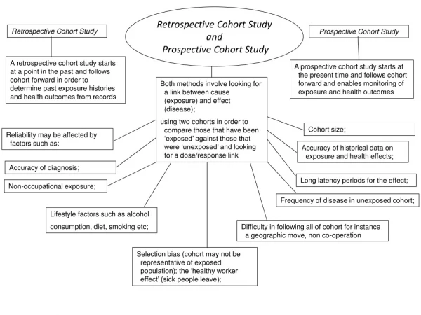
Types of Cohort Present Future Past Concurrent Cohort Followed into future Assembled now Assembled from past records Historical Cohort Followed till now Exposure and outcome Retrospective Cohort
Analysis of Cohort Studies Exposed Time Diseased (n=39) Healthy n = 30 000 Not exposed Diseased (n=6) Healthy n = 60 000
Modifiable risk factors Non-modifiable risk factors -Medication: Corticosteroids - Bone-related factors: BMD, bone strength indice… - Fall and fall-related factors - Prior fracture - Lifestyle: smoking, alcohol - Advancing age - Family history - Genetics Fracture Intervention strategies Identify high-risk group
Prospective Cohort Study • Basal cohort(s) • Sampling from defined population, or • Stratified assembly, or • Matched assembly • Observation for defined period under specified observational protocol • Time of data collection: prospective vs. Retrospective cohort studies
Factors in Prospective cohort study • Event (e.g. disease) • Person at risk, population at risk • Person-years
Population at risk (N=200)
Week 1 O O
Week 2 O O O O O
Week 3 O O O O O O O
Person-time • Person-time = # persons x duration 1 o 2 x 2 4 3 4 4 8 5 2 0 2 4 6 8 Time (week) Incidence rate (IR). During (2+4+4+8+2)=20 person-years, there were 2 incident cases: IR = 2/20 = 0.1
Estimation of Incidence Rates • Consider a study where P patient-years have been followed and N cases (eg deaths, survivors, diseased, etc.) were recorded. • Assumption: Poisson distribution. • The estimate of incidence rate is: I = N / P • Standard error of I is: • 95% confidence interval of “true” incidence rate: I+ 1.96 x SD(I)
Relative Risk • Relative risk (RR): Incidence rate of ischemic heart disease (IHD) <2750 kcal >2750 kcal ______________________________________________________________ Person-years 1858 2769 New cases 28 17 ______________________________________________________________ Estimate rate 15.1 6.1 SD of est. rate 2.8 1.5 • L = log(RR) = 0.908 • Standard error of log(RR) • 95% of L: L ±1.96xSE = 0.908 ± 1.96x0.3075 = 0.3055, 1.51 • 95% of RR: = exp(0.3055), exp(1.51) = 1.36, 4.53
Analysis of Difference in Incidence Rates • Difference: D = 15.1 – 6.1 = 8.93 Incidence rate of ischemic heart disease (IHD) <2750 kcal >2750 kcal ______________________________________________________________ Person-years 1858 2769 New cases 28 17 ______________________________________________________________ Estimate rate 15.1 6.1 SD of est. rate 2.8 1.5 • Standard error (SE) of D • 95% of D = D ±1.96xSE = 8.93 ± 1.96x0.032 = 3.65, 14.2
Logistic Regression Analysis using R fracture <- read.table(“fracture.txt”, header=TRUE, na.string=”.”) attach(fulldata) results <- glm(fx ~ bmd, family=”binomial”) summary(results) Deviance Residuals: Min 1Q Median 3Q Max -1.0287 -0.8242 -0.7020 1.3780 2.0709 Coefficients: Estimate Std. Error z value Pr(>|z|) (Intercept) 1.063 1.342 0.792 0.428 bmd -2.270 1.455 -1.560 0.119 (Dispersion parameter for binomial family taken to be 1) Null deviance: 157.81 on 136 degrees of freedom Residual deviance: 155.27 on 135 degrees of freedom AIC: 159.27
Incidence Density Number of new casesID = ––––––––––––––––––– Population time Number of new cases 7ID = ––––––––––––––––––– = –––––– Population time ?
Incidence Rate • Population time at risk: • 200 people for 3 weeks = 600 person-wks • But 2 people became cases in 1st week • 3 people became cases in 2nd week • 2 people became cases in 3rd week • Only 193 people at risk for 3 weeks
Incidence Rate • Population-time: • 2 people who became cases in 1st week were at risk for 0.5 weeks each = 2 @ 0.5 = 1.0 • 3 people who became cases in 2nd week were at risk for 1.5 weeks each = 3 @ 1.5 = 4.5 • 2 people who became cases in 3rd week were at risk for 2.5 weeks each = 2 @ 2.5 = 5.0 • Non-cases = 193 @ 3 = 579 • TOTAL POPULATION – TIME = 589.5 Person-weeks • Incidence rate: 7 ID = –––––– = 0.0119 cases / person-wk 589.5 average over 3 weeks
Incidence Proportion Number of new casesCI = ––––––––––––––––––– Population at risk 73-week CI = –––– = 0.035 200
Summary of Cohort Study’s Results Relative risk (RR) = I1 / I2
Person-time • Person-time = # persons x duration 1 2 2 4 3 4 4 8 5 2 0 2 4 6 8 Time Incidence rate (IR). During (2+4+4+8+2)=20 person-years, there were 2 incident cases: IR = 2/20 = 0.1
Estimation of Incidence Rates • Consider a study where P patient-years have been followed and N cases (eg deaths, survivors, diseased, etc.) were recorded. • Assumption: Poisson distribution. • The estimate of incidence rate is: I = N / P • Standard error of I is: • 95% confidence interval of “true” incidence rate: I+ 1.96 x SD(I)
Relative Risk • Relative risk (RR): Incidence rate of ischemic heart disease (IHD) <2750 kcal >2750 kcal ______________________________________________________________ Person-years 1858 2769 New cases 28 17 ______________________________________________________________ Estimate rate 15.1 6.1 SD of est. rate 2.8 1.5 • L = log(RR) = 0.908 • Standard error of log(RR) • 95% of L: L ±1.96xSE = 0.908 ± 1.96x0.3075 = 0.3055, 1.51 • 95% of RR: = exp(0.3055), exp(1.51) = 1.36, 4.53
Analysis of Difference in Incidence Rates • Difference: D = 15.1 – 6.1 = 8.93 Incidence rate of ischemic heart disease (IHD) <2750 kcal >2750 kcal ______________________________________________________________ Person-years 1858 2769 New cases 28 17 ______________________________________________________________ Estimate rate 15.1 6.1 SD of est. rate 2.8 1.5 • Standard error (SE) of D • 95% of D = D ±1.96xSE = 8.93 ± 1.96x0.032 = 3.65, 14.2
Logistic Regression Analysis using R fracture <- read.table(“fracture.txt”, header=TRUE, na.string=”.”) attach(fulldata) results <- glm(fx ~ bmd, family=”binomial”) summary(results) Deviance Residuals: Min 1Q Median 3Q Max -1.0287 -0.8242 -0.7020 1.3780 2.0709 Coefficients: Estimate Std. Error z value Pr(>|z|) (Intercept) 1.063 1.342 0.792 0.428 bmd -2.270 1.455 -1.560 0.119 (Dispersion parameter for binomial family taken to be 1) Null deviance: 157.81 on 136 degrees of freedom Residual deviance: 155.27 on 135 degrees of freedom AIC: 159.27
Dubbo Osteoporosis Epidemiology Study • 1989 – 1993: • Recruit 3000 individuals • Measure bone mineral density (BMD) • Classified BMD into normal and osteoporosis • 1989 – 2005: • Record the number of fractures • Analysis of association between BMD and fracture
Dubbo Osteoporosis Epidemiology Study 1287women Low BMD 345 (27%) Not Low BMD 942 (73%) Fx = 137 (40%) No Fx = 208 (60%) Fx = 191 (20%) No Fx = 751 (80%) 42%
Direct calculation of incidence Time sequence can be established Different outcomes for one agent can be determined Advantages and Disadvantages of Cohort Studies Disadvantages Advantages • Large numbers to be measured over a long time • Subclinical disease may escape diagnosis