Download
1 / 49
490 likes | 574 Views
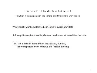
Lecture 25. Some Simple Control Examples. in which we enlarge upon the simple intuitive control we’ve seen. We generally want a system to be in some equilibrium state. If the equilibrium is not stable, then we need a control to stabilize the state.

E N D
Lecture 25. Some Simple Control Examples in which we enlarge upon the simple intuitive control we’ve seen We generally want a system to be in some equilibrium state If the equilibrium is not stable, then we need a control to stabilize the state
Dear Professor Gans,Did you know that your students can download Mathematica from us at Wolfram and use it on personal machines as well as on campus? Several faculty have told us that because our convenient download site now provides ubiquitous access, they have started to require more projects that use Mathematica. So if you or your students aren't yet using Mathematica, let me know and I'll get you details.And if you're already using Mathematica through the site license, don't forget to request your free staff home-use license:http://url.wolfram.com/2GUohz3K/Best regards,Katherine BautistaSenior Academic Program ManagerWolfram Research, Inc.katherine_bautista@wolfram.comhttp://www.wolfram.com
Last time we looked at an electric motor attached to a disk and set it up as a second order system or
Suppose we want the angle to be fixed at π/3 The desired state satisfies the differential equations with no input voltage
We can write the differential equations for the primed quantities We want the perturbations to go to zero Is the homogeneous solution stable? What are the eigenvalues of A?
There is one stable root and one marginally stable root. The homogeneous solution is
If the initial value of q’is not equal to its desired value then it will not decay. The problem as posed is satisfied for everything equal to zero but that’s not good enough We need control. If q’ is too big we want to make it smaller and vice versa Let’s look at this in block diagram mode
Here’s a block diagram representation of the differential equations open loop - + e q’ w’
We can close the loop by feeding the q’ signal back to the input closed loop - - w’ q’ feedback loop
We’ve gone from an inhomogeneous set of equations to a homogeneous set This what closing the loop does; there’s no more undetermined external input. We want q and w to go to zero, and that will depend on the eigenvalues of the new system
This will converge to zero for any positive g Let’s put in some numbers: K = 0.429, R = 2.71, Ix = 0.061261 (10 cm steel disk) We are overdamped for small g and underdamped for large g We can get at the behavior by applying what we know about homogeneous problems
The eigenvectors I will select g = 0.2379 (to make some things come out nicely) This leads to s = -0.544 ± 0.544j
The homogeneous solution is With the numbers we have
At t = 0, we have A little algebra Now we have the complete solution in terms of the initial conditions
Let’s plot this and see what happens for q’0= π/3 and w’0= 0
Now let’s take a closer look at the cruise control we started with Tuesday evening This is a much harder problem than the one we just worked We designed a simple control to eliminate starting error — cruise control is meant to eliminate an ongoing error, an unknown external force Recall the abstract block diagram
CRUISE CONTROL desired speed GOAL: SPEED INVERSE PLANT nominal fuel flow Actual speed + + PLANT: DRIVE TRAIN Input: fuel flow - - error disturbance Feedback: fuel flow adjustment CONTROL
We have some open loop control — a guess as to the fuel flow, the nominal fuel flow We have some closed loop control — correct the fuel flow if the speed is wrong We have disturbances that will make the speed wrong if we don’t do something about them We need to make a model, and then try to control the model Ultimately we’d want to run the model control on a simulation
disturbance simple first order model open loop part divide the force control part linearize and the goal is to make v’ go to zero
Let’s say a little about possible disturbances hills are probably the easiest to deal with analytically mgsinf f I’ll say more as we go on
The open loop picture + + f’ v’ 1/m -
I’m not in a position to simply ask f to cancel h(t) (because I don’t know what it is!) I want some feedback mechanism to give me more fuel when I am going too slow and less fuel when I am going too fast I use K for gain here This is what we just did for the motor-disk system
The closed loop picture The open loop picture + + - f’ v’ 1/m - control feedback Note that this feedback really isn’t doing anything new — we already have negative feedback from the speed caused by air drag
But let’s carry on for a moment From the last lecture So we have Solution
We do not need this whole apparatus to get a sense of how this works Consider a hill, for which s(t) is constant, call it s0 We can find the particular solution by inspection The homogeneous solution decays, and we see that we have a permanent error in the speed The bigger K, the smaller the error, but we can’t make it go away (and K will be limited by physical considerations in any case)
What we’ve done so far is called proportional (P) control We can fix this problem by adding integral (I) control. There is also derivative (D) control PID control incorporates all three types, and you’ll hear the term We won’t do D control today — it doesn’t buy us much for this problem
Add a variable and its ode Let the force depend on both variables Then
Look at the block diagram for this the red part is new f’ - y’ v’ 1/m - “natural” feedback + control feedback +
Convert to state space We remember that x denotes the error so the initial condition for this problem is y’= 0 = v’
The homogeneous solution and we see that it will decay if k2 >0
What happens now when we go up a hill? We can now let the displacement take care of the particular solution
Wait a minute here! What’s going on!? Have I pulled a fast one? No, let’s look at it more carefully using some of our mathematical development
Method 1 go “backwards” to get a second order ode — a familiar one The particular solution is constant, as we have seen Let’s look at the homogeneous solution
Method 1 so the system will be underdamped if and in that case we have
Method 1 Initial conditions: y’H+ y’P= 0, v’H+ v’P= 0 from which and its derivative clearly decays, leaving no permanent error in speed
Method 2 and we can use the state transition matrix We’ll need numbers to make that work: let k1 = 1 = k2 This satisfies the condition for an underdamped response And let g = 1, which we can do by choosing a time scale
Method 2 The eigenvalues and eigenvectors are We see that the system is stable, as we expected
Method 2 The state transition matrix is so that the response to any h(t) is given by
Suppose we have a more varied terrain? Let scaled response
The control still works very well, and tracks nicely once it is in place. Let’s look at a much more complicated roadway
The scaled response looks like the scaled forcing and the velocity error is minuscule — this really works
What did we do here? We started with a one dimensional system — and tried to find a force to cancel and exterior force That didn’t work We added a variable to the mix found a new feedback got the velocity to be controlled at the expense of its integral about which we don’t care very much
Look at the block diagram for this the red part is new f’ - y’ v’ 1/m - “natural” feedback + control feedback +
We need to say more about state transition matrices We will discover that the simple feedback games we’ve just played don’t always work We will learn how to control more complicated mechanisms and get the to do more complicated things