Download

1 / 17
170 likes | 185 Views
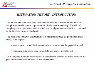
Parameter Estimation. Covered only ML estimator. Given an i.i.d data set X, sampled from a distribution with parameters q , we would like to determine these parameters, given the samples. Once we have those, we can estimate p(x) for any given x, given the known distribution.

E N D
Parameter Estimation Covered only ML estimator
Given an i.i.d data set X, sampled from a distribution with parameters q, we would like to determine these parameters, given the samples. • Once we have those, we can estimate p(x) for any given x, given the known distribution. • Two approaches in parameter estimation: • Maximum Likelihood approach • Bayesian approach (will not be covered in this course)
Examples: Bernoulli/Multinomial • Bernouilli:Binary random variable x may take one of the two values: • success/failure, 0/1 with probabilities: • P(x=1)=po • P(x=0)=1-po • Unifying the above, we get: P (x) = pox(1 – po )(1 – x) • Note that the single formula helps rather than having two separate formulas (one for x=1 and one for x=0) • Given a sample set X={x1,x2,…}, we can estimate p0 using the ML estimate by maximizing the log-likelihood of the sample set: Log likelihood (po) : log P(X|po) = log ∏tpoxt(1 – po )(1 – xt)
Examples: Bernoulli log L=log P(X|po) = log ∏tpoxt(1 – po )(1 – xt) t=1, N and xtin {0,1} = St log ( poxt(1 – po )(1 – xt) ) = St log poxt + log(1 – po )(1 – xt) = St(xt log po+ (1 – xt) log(1 – po ) ) In solving for the necessary condition for extrema, we must have dlogL/dpo = 0. Take derivative, set to 0 and solve...: dlogL/dpo = Stxt .(1/po)+ St(1 – xt) .1/(1 – po ).-1 = 0 Remember: derivative of log x is 1/x. • Stxt . (1/po) = St (1 – xt) . 1/(1 – po ) => Stxt = St po = Npo => Stxt . (1 – po ) = St (1 – xt) . po => MLE: po = ∑txt /N • Stxt -po Stxt =St po –po St xt
Examples: Bernoulli You can also arrive to the same conclusion (easier) by finding the likelihood of the parameter p0, when observing the number of successes, z, of the random variable x, where: z = ∑txt z ~ Binomial (N,p0) when x ~ Bernoulli (p0) P(z) = (N choose z) p0z (1-p0)(N-z) --------------------------------------------------------------------------------------------------- Example: Assume we got HTHTHHHTTH (6H, 4T in 10 i.i.d. coin toss: z=6) Log L (p0) = z logp0 + (N-z) log(1-p0) = 0 Plug z, set to 0 and solve for p0 p0 = 6/10
Examples: Categorical • Bernoulli -> Binomial • Categorical –> Multinomial • Categorical:K>2 states,xiin {0,1} • Instead of two states, we now have K mutually exclusive and exhaustive events, with probability of occurence of piwhere Sipi = 1. • Ex. A dice with 6 possible outcomes. • P(x=1)=p1 x = [1 0 0 0 0 0] = [x1 ... x6] • P(x=2)= p2 .... P(x=6)= p6 • Unifying the above, we get: P (x) = ∏ipixiwhere xi is 1 if outcome is state i0 otherwise Similar to p(x) = px(1-p)(1-x) when there were two possible outcomes for x log L(p1,p2,...,pK|X) = log ∏t ∏ipixit MLE: pi = ∑txit / N Ratio of experiments with outcome of state i (e.g. 60 dice throws, 15 of them were 6 p6 = 15/60
Gaussian Parameter Estimation Likelihood function Assuming iid data
Reminder • In order to maximize or minimize a function f(x) w.r.to x, • we compute the derivative df(x)/dx and set to 0, since a necessary condition for extrema is that the derivative is 0. • Commonly used derivative rules are given on the right.
Maximum (Log) Likelihood for a 1D-Gaussian In other words, maximum likelihood estimates of mean and variance are the same as sample mean and variance.