Download
1 / 55
550 likes | 647 Views
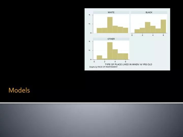
Models. Administrative Stuff:. Anna’s Office Hours Tuesday after class: in the Co-lab Friday 10-11am: rm 107. Making Sense of Overwhelming Data.

E N D
Administrative Stuff: • Anna’s Office Hours • Tuesday after class: in the Co-lab • Friday 10-11am: rm 107
Making Sense of Overwhelming Data “Today companies like Google, which have grown up in an era of massively abundant data, don't have to settle for wrong models. Indeed, they don't have to settle for models at all. –Chris Anderson”
The Scientific Method is Built Around the Idea of Constructing and Testing Models…So What is a Model? X ~ N(0,1)
George Box, a famous statistician, on “worrying selectively”: “ Since all models are wrong the scientist must be alert to what is importantly wrong. It is inappropriate to be concerned about mice when there are tigers abroad. ”
George Box on parsimony: “ Since all models are wrong the scientist cannot obtain a “correct” one by excessive elaboration. On the contrary following William of Occam he should seek an economical description of natural phenomena. Just as the ability to devise simple but evocative models is the signature of the great scientist so overelaboration and overparameterization is often the mark of mediocrity. ”
Simple Example of a Type of Overelaboration: Overfitting…or “memorizing the data” (From Lee et al. 2006, “Overfitting Control for Surface Reconstruction”)
Non Normal Distributions • Skewness • Kurtosis Playtykurtic Leptokurtic
Describing Distributions • Central Tendency • Some way of “typifying” a distribution of values, scores, etc. • Mean • sum of scores divided by number of scores • Median • middle score, as found by rank • Mode • most common value from set of values • In a normal distribution, all 3 measures are equal. Image: http://thenormalgenius.blogspot.com
Special Features of the Mean • Sum of the deviations from the mean of all scores = zero. • It is the point in a distribution where the two halves are balanced.
Using Central Tendencies in Recoding Variables • “splitting” metric variables into binary variables • High/Low (mean or median) • Most common, least common (mode) • “collapsing” variables (less from more) • Groups of scores in different ranges above and below the mean
Dispersion • Range • Overall measure of distance between all values in a variable. • Variance • Computed as the average squared deviation of each value from its mean • Standard Deviation • A statistic that describes how tightly the values are clustered around the mean. Both of these distributions have same mean, but top figure has greater dispersion.
Sum of Squares and Variance • Consider this example: number of words in a sample of your own emails. • We can use the mean as a statistical model– it is a hypothetical value that describes something of interest. • The word count in each individual email will likely differ a little from the mean. This is error. • By squaring the errors and then taking the sum, we get the sum of squared errors, or SS. • We can divide the SS by N-1 to account for the sample size. This value is the variance. Equation for variance
Standard Deviation (S.D.) • S.D is the square root of the variance. • S.D. is in same units as the original measure. • If a constant is added to all scores, it has no impact on S.D. • If a constant is multiplied to all scores, it will affect the dispersion (S.D. and variance) S = standard deviationX = individual scoreM = mean of all scoresn = sample size (number of scores)
Common Data Representations • Histograms • Simple graphs of the density or frequency • With density, area comes out in percent and total area = 100% • Box Plots • Yet another way of displaying dispersion. Provides a lot of information in one graphic.
Why Sum of Squares? • Say that we want to minimize the sum of squares error about an estimate, x • To minimize this, we use the first order condition: • In other words, the sum of squares is the error that is minimized by the mean
Why N-1? • Variance is the average squared error • For a whole population, we would simply compute • For a sample, the sample mean is shifted towards our sampled data points, which lowers our calculation of variance. • To correct this, we compute mean sample mean
Frequency Distributions and Probability • Probability corresponds to area under frequency distribution • Often, we don’t know the frequency distribution, but have reason to believe it’s approximately normal
The z-score and the normal distribution(z-scores are also called standard units) • Standardizing a group of scores changes the scale to one of standard deviation units. • Allows for comparisons with scores that were originally on a different scale. Or…
z-scores (continued) • Tells us where a score is located within a distribution. • Properties • The mean of a set of z-scores = zero • The variance and standard deviation of a set of z-scores = 1.
Using z-scores: Area under the normal curve • Example, you have a variable x with mean of 500 and S.D. of 15. How common is a score of 525? • Z = 525-500/15 = 1.67 • A z-statistic of 1.67 (as found in a z-score table), we find that the proportion of scores less than our value is .9525. • Or, a score of 525 is very rare. In very specific terms, our specified score is larger than .9525 of the population.
Other sources of error • Chance: expected error from random fluctuation, factors outside model • Individual measurement = exact value + chance error • Bias: systematic error, net positive or negative expected value • Recording: isolated errors • Can cause outliers - extreme measures far outside the normal curve 3 Major Sources of Error
Why spend so much time on the normal distribution? • For some statistical tests, our variables may need to meet the assumption of normality. • A key assumption for many variables is that the means of samples are normally distributed. • We are especially interested in the normal distribution as it relates to sampling distributions.
Sampling Variation and Sampling Distributions • Sampling Variation • If we take different samples from the same population, the means for each sample will likely be different. • Sampling Distribution • This is the frequency distribution of sample means (or any statistic that we want to estimate for that matter) obtained from the same population. • In general, we don’t actually know the sampling distribution, but may have reason to think it’s normal
Two Big Laws of Asymptotics • The Law of Large Numbers: • For a population with mean μ, the sample mean approaches the population mean • Technically, the sample mean is a consistent estimator of μ: Prob(|Y – μ| > ε ) -> 0 as n -> ∞ for anyε • This means that we can use the sample mean as a sensible estimator for the population mean. _ 1 n ∑ _ Yn = Yi
How Good an Estimator is the Sample Mean? • In other words, how spread out is the sampling distribution about the true population mean? • We can compute the standard deviation of the sampling distribution – this is called the standard error. • Large samples give us more accuracy • In other words, small samples only allow us to uncover large effects
The Difference between Standard Deviation and Standard Error • Standard Deviation • Measures spread of any distribution • Especially spread of population parameters • Standard Error • Standard deviation of a sampling distribution • more commonly, estimates of that standard deviation • Applies when we want to know how good our sample parameter is an an estimate for a population parameter Graphics: Wikipedia
Two Big Laws of Asymptotics • Central Limit Theorem • Even for small samples, if errors can be viewed as a sum of many independent random effects, individual scores will tend to be normally distributed. • This assumption is often questionable • The mean of a large number of independent and identically-distributed random variables will be approximately normally distributed
What does the Central Limit Theorem Imply? • We are using a sample to estimate the mean for an entire population. The Central Limit Theorem tells us about how that estimate is distributed. • This lets us to figure out how confident we should be in our estimate, or how close the actual value is likely to be. • In other words, it allows us to do statistics on statistics • Or at least statistics on estimators • The LLN and the Central Limit Theorem rely on properties of the sample mean, but they often apply to estimators in general.
An example* Note: reproduced from Karl Whelan’s class notes