Download
1 / 43
600 likes | 976 Views
F. Applications of Derivatives. Calculus 30 C30.6 Demonstrate understanding of the application of derivatives to solve problems including: optimization rates of change related rates. 1. Rate of Change. C30.6

E N D
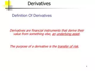
F. Applications of Derivatives Calculus 30 C30.6 Demonstrate understanding of the application of derivatives to solve problems including: optimization rates of change related rates.
1. Rate of Change • C30.6 • Demonstrate understanding of the application of derivatives to solve problems including: optimization rates of change related rates.
1. Rate of Change • We saw in unit D that the slope of the tangent line represents the rate of change of y compared to x at a specific value of x.
Assignment • Ex. 6.1 (p. 264) #1-8
2. Distance, Velocity and Acceleration • C30.6 • Demonstrate understanding of the application of derivatives to solve problems including: optimization rates of change related rates.
2. Distance, Velocity and Acceleration • Distance, velocity, and acceleration are most often thought of as quantities used in physics, but calculus can be used to make the calculations of these quantities easier.
Note that the average velocity and acceleration are found by calculating the slope of the secant line between two points. • Instantaneous velocity is actually the derivative of distance (position). • Instantaneous acceleration is actually the derivative of velocity.
Assignment • Ex. 6.2 (p. 271) #1-7
3. Optimization Problems • C30.6 • Demonstrate understanding of the application of derivatives to solve problems including: optimization rates of change related rates.
3. Optimization Problems • The power of the derivative will be made apparent in this section. • By determining the global maximum or global minimum of a function on a given domain, we can solve many interesting and practical problems.
Problem Solving Tips • Until you have actually tried to solve some optimization problems, the following suggestions may be meaningless to you. • Once you become bogged down, however, you may wish to re-examine these tips more carefully.
1. Understand the Problem • Optimization problems often appear in the form of a word problem. • It is most important that you read the problem over until you have a clear idea of what it is you are being asked to maximize or minimize.
2. Draw a Diagram • Many optimization problems require a diagram. Label your diagram carefully with all given dimensions. • Use variables to label dimensions that you do not know. • Using meaningful variables, such as h for height and r for radius can be very helpful.
3. Determine the Function • Set up a function that gives an expression for the quantity you are trying to optimize. • Initially, the function may be in terms of more than one variable. Read your problem carefully and re-examine your diagram to see any interrelations between your variables. • You must write your optimization function in terms of only one variable before you can proceed.
4. Determine the Domain of the Function • Read the problem carefully to determine the domain of the function. • The domain becomes relevant as you proceed to the next step.
5. Determine the Global Maximum or Minimum • Evaluate the function at the endpoints of the domain as well as the critical numbers.
6. Answer the Question • Be sure to answer the question that was asked.
Assignment • Ex. 6.3 (p. 277) #1-14, 15-27 odds
4. Related Rates (Sides of Triangles) • C30.6 • Demonstrate understanding of the application of derivatives to solve problems including: optimization rates of change related rates.
4. Related Rates (Sides of Triangles) • Some office buildings have glass-enclosed elevators and elevator shafts. Thus, it is possible to observe people moving up and down the building by standing at ground level. • Suppose your friend gets into the elevator and proceeds to the twenty-fifth floor of the building. If you are standing 30m away from the base of the elevator, then as your friend proceeds up at a uniform rate, the distance between you and your friend is increasing. • The rate at which the distance between the two of you is increasing is dependent at the rate at which the elevator is moving. One rate of change is related to another. This is an illustration of what is meant by a related rate.
Background Information a) Recall that the derivative,, gives us a measure of the rate of change of y relative to x. • If t represents time, and y represents a length or distance, then gives us a measure of the rate of change in the length of y relative to time. Thus , would have units such as cm/s, m/s, or km/h.
b) We will use implicit differentiation and the chain rule throughout this section. • Recall that the derivative of is , whereas the derivative of with respect to x is . • Similarly, the derivative of with respect to t is , and the derivative of with respect to t is .
c) We see that the end result is obtained by “differentiating normally, then adding the appropriate tag-a-long.”
Example Differentiate each expression with respect to time, t.
What follows is a set of suggestions that will help you in solving related rate problems.
1. Read the problem, carefully. 2. Make a well labeled diagram that shows all of the variables and constants involved. This will be the “whenever diagram.” 3. Write an equation that shows the relationship among the quantities involved in the problem. 4. Implicitly differentiate the equation developed above relative to time, t.
5. Substitute the given “when” information into the differentiated result, using the appropriate units. • It is most likely that you will have to do a side calculation to determine the value of one of your variables. • It may be necessary to draw a new diagram replacing some of the variables from the “whenever diagram” with values given in the problem. • After substitution, you should find that there is only one unknown remaining, the one you need to solve for.
6. Solve for the remaining unknown. 7. Form your conclusion.
Assignment • Ex. 6.4 (p. 284) #1-12
5. Related Rates (Areas and Volumes) • C30.6 • Demonstrate understanding of the application of derivatives to solve problems including: optimization rates of change related rates.
5. Related Rates (Areas and Volumes) • The last section on related rates dealt with right triangles. This section changes the focus onto areas and volumes of figures. • The steps involved in solving these types of problems are very similar. Well-labeled diagrams are critical and side calculations will be required.
Note * • A list of formulas can be found on pp445-448 of your text.
Assignment • Ex. 6.5 (p.290) #1-20 odds