Download
1 / 27
280 likes | 529 Views
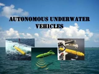
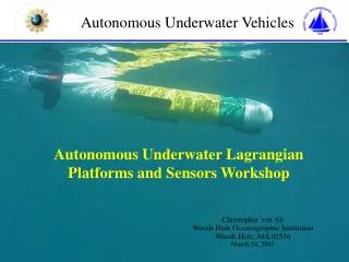
Path Planning of Autonomous Underwater Vehicles for Adaptive Sampling. DEAS Group Meeting Presentation Namik Kemal Yilmaz April 6, 2006. Ocean Forecasting. Ocean forecasting is essential for effective and efficient operations at sea. It is used for: Military operations

E N D
Path Planning of Autonomous Underwater Vehicles for Adaptive Sampling DEAS Group Meeting Presentation Namik Kemal Yilmaz April 6, 2006
Ocean Forecasting • Ocean forecasting is essential for effective and efficient operations at sea. It is used for: • Military operations • Coastal zone management • Scientific research • State variables to be forecasted: • Temperature • Salinity • Current velocity • Plankton concentration • Nutrient concentration • Fish concentration • Pollution • Sound speed
Adaptive Sampling • There exists a routinecomponent for observations which collects data from a particular region. • Adaptive sampling is a method which aims to the improvement of the forecast results by deploying some additional assets to gather more accurate data in critical regions. • The trajectory of this additional component needs to be planned continuously. It needs to adapt to changing conditions, therefore named “adaptive”. • Forecasting systems such as “Error Subspace Statistical Estimation” (ESSE) or “Ensemble Transform Kalman Filter” (ETKF) techniques provide both estimates of the states and the uncertainty on the state estimate. • Uncertainty fields created by these techniques can be used for the purpose of adaptive sampling.
Adaptive Sampling-Summary Maps * • Summary maps represent the amount of total improvement on a given field as a function of measurement location. • Path planning is done manually. Paths are either created manually or chosen from a set of pre-designed paths. • Use of pre-designed paths limit the quality of adaptive path planning. • The multi-vehicle case is handled by “serial targeting”. • Find the best path for first vehicle. • Assimilate the fictitious observations made by the first vehicle using ESSE or ETKF. • Using the updated summary map, find the path of the second vehicle. • The technique does not deal with more complicated scenarios where inter-vehicle interactions and other mission constraints are involved. * S. J. Majumdar, C. H. Bishop, and B. J. Etherton. Adaptive sampling with the ensemble transform Kalman filter. Part II: Field program implementation. Monthly Weather Review, 130:1356–1369, 2002.
Problem Statement • Given an uncertainty field, find the paths for the vehicles in the adaptive sampling fleet along which the path integral of uncertainty values will be maximized. Also constraints such as: • Vehicle range • Desired motion shape • Inter-vehicle coordination • Collision avoidance • Communication needs must be satisfied. • Also there might be multiple days in succession involved in the adaptive sampling mission. The optimality must be sought over a time window. This is named the “time-progressive” case. • Global optimality in the spatial and time sense must be satisfied. • The fields are neither concave nor convex. • Increases the challenge.
A Short Introduction to Optimization Methods • A generic optimization problem can be written as Types of different optimization problems: • Non-linear programming problem • Linear programming problem • Integer programming problem • Mixed integer programming (MIP) problem
Mixed Integer Programming (MIP) Solution Methods Comparison of some solution methods
Network-Based MIP Formulation • Needs processing of huge matrices before each run • Complicated to include diagonal moves • Costly to make modifications on the formulation and add new constraints • Does not handle time-progressive case
New Mixed Integer Programming (MIP) Method N: Number of path points P: Total number of vehicles Variables: xpi and ypi where i є [1,…,N], and p є [1,…,P]. 1≤ xpi ≤maxX 1≤ ypi ≤maxY Decision Variables: bpij ,t1pij , t2pij , t3pij where i є [1,…,N], and p є [1,…,P], and j є [1,…,4], bpij ,t1pij ,t2pij ,t3pijє{0,1}
Autonomous Ocean Sampling Network (AOSN)& Communication Constraints * • Different Scenarios Based on Communication Needs: • Communication with a ship. • Communication with a shore station. • Communication with buoys. * Adapted from Tom B. Curtin, James G. Bellingham, J. Catipovic, and D. Webb. “Autonomous Oceanographic Sampling Networks”. Oceanography, 6(3), 1993.
Communication with a Ship • Constraints for collision avoidance between the ship and the AUVs • Communication via acoustic link • AUV must always lie within a defined vicinity of the ship (continuous shadowing) • If the vehicle needs to return to the ship
Communication with a Ship • Communication via radio link • AUV must come within a vicinity of the ship only at the end of the mission to transfer data. • If the vehicle needs to lie in a tighter vicinity of the ship at the terminal path point Only these equations apply !
Communication with a Shore Station and AOSN • Communication with an AOSN • Communication with a shore station • We have “M” buoys and only one AUV can dock at a given buoy. If the AUVs need to return to the shore station: At most one AUV can dock at a given buoy
Results for a Single Vehicle Range:10 km Range:15 km Range:20 km Range:25 km Starting Coordinates: x=7.5km; y=21km
Range:30 km Range:35 km Solution time as a function of range on a Pentium 4- 2.8Ghz computer with 1GB RAM. • Exponential growth is observed as expected • The solution times are acceptable Results for a Single Vehicle
Number of path points: 8 Range1: 15 km Range2: 14 km Number of path points: 10 Range1: 16.5 km Range2: 18 km Number of path points: 13 Range1: 22.5 km Range2: 24 km Solution time as a function of path-points on a Pentium 4- 2.8Ghz computer with 1GB RAM Results for Two Vehicles
Results for Vehicle Number Sensitivity Number of path points: 8 1 vehicle 2 vehicles 3 vehicles 4 vehicles 5 vehicles Solution time as a function of vehicle number on a Pentium 4- 2.8Ghz computer with 1GB RAM
Time Progressive Path Planning • When path planning needs to be performed over multiple days, the formulation must be extended to combine information from all days under consideration. D: Total Number of Days Single Day Formulation Time Progressive Formulation
Illustrative Results for Time-Progressive Path Planning Paths Generated for Day 1 Paths Generated for Day 2 Number of Path Points= 8 Solution Time: 179 sec
An Example Solved by the Dynamic Method • It is a 3 day long mission: August 26-28, 2003. • 2 consecutive 2 day time-progressive and 1 single day problems are solved. • Measurements are assimilated using Harvard Ocean Prediction System (HOPS). Phase 1 August 26&27 Optimization Code HOPS Solution on Coarse (Half-Size) Grid for Day 2 (August 27) Solution on Coarse (Half-Size) Grid for Day 1 (August 26) Solution on Full Size Grid for Day 1 (August 26) Solution on Full Size Grid for Day 2 (August 27)
An Example Solved by the Dynamic Method Phase 2 August 27&28 Solution on Full Size Grid for Day 1 (August 27) Solution on Full Size Grid for Day 2 (August 28) Phase 3 August 28 Solution on Full Size Grid for Day 1 (August 28)
Comparison of Results of the Dynamic Method with Results without Adaptive Sampling Results Without Adaptive Sampling: August 27 August 28 August 26 Dynamic Case Results: August 27 August 28 August 26
Recommendations for Future Work • Devise methods to automatically determine the optimal values of some of the problem parameters based on a given uncertainty field, e.g. inter-vehicle distance, starting point seperation etc.. • Approximate the uncertainty prediction/assimilation by a linear operator and embed this operator into the optimization code. It will help: • To establish a link between the choice of measurement locations and its effect on the following day’s uncertainty field. • To improve the quality of path planning as a result. • Current Work: • Working on two journal and one conference papers. • Investigating the feasibility of implementing a (simplified) version of the MILP formulation on MATLAB.