Download
1 / 46
490 likes | 801 Views
Boundary Layer Verification. ECMWF training course April 2013 Maike Ahlgrimm. What does the BL parameterization do?. Attempts to integrate effects of small scale turbulent motion on prognostic variables at grid resolution. Turbulence transports temperature, moisture and momentum (+tracers).

E N D
Boundary Layer Verification ECMWF training course April 2013 Maike Ahlgrimm
What does the BL parameterization do? Attempts to integrate effects of small scale turbulent motion on prognostic variables at grid resolution. Turbulence transports temperature, moisture and momentum (+tracers). Ultimate goal: correct model output
Which aspect of the BL can we evaluate? large scale • 2m temperature/humidity • Depth of BL • Diurnal variability of BL height • Structure of BL (temperature, moisture, velocity profiles) • Turbulent transport within BL • Boundaries: entrainment, surface fluxes, clouds etc. small scale Chandra et al. 2010
Part 1 Depth of the boundary layer
Boundary Layer Height from Radiosondes How to define the BL top? Heat and moisture well-mixed in BL (convective BL) Flow transitions from turbulent to laminar at BL top (any BL) Three methods: • Heffter (1980) (1) • Liu and Liang Method (2010) (1+) • Richardson number method (2) normalized BL height Figure: Martin Köhler Must apply same method to observations and model data for equitable comparison! For a good overview, see Seidel et al. 2010
Heffter method to determine PBL height Potential temperature gradient Potential temperature gradient exceeds 0.005 K/m Pot. temperature change across inversion layer exceeds 2K • Note: • Works on convective BL only • May detect more than one layer • Detection is subject to smoothing applied to data Potential temperature Sivaraman et al., 2012, ASR STM poster presentation
Liu and Liang method First, determine which type of BL is present, based on Θ difference between two near-surface levels Liu and Liang, 2010
Liu and Liang method: convective BL For convective and neutral cases: Lift parcel adiabatically from surface to neutral buoyancy (i.e. same environmental Θ as parcel), and Θ gradient exceeds minimum value (similar in concept to Heffter). Parameters δs,δ u and critical Θ gradient are empirical numbers, differing for ocean and land. Liu and Liang, 2010
Liu and Liang method: stable BL Stable case: Search for a minimum in θ gradient (top of bulk stable layer). If wind profile indicates presence of a low-level jet, assign level of jet nose as PBL height if it is below the bulk layer top. Advantage: Method can be applied to all profiles, not just convective cases. Liu and Liang, 2010
Turbulent kinetic energy equation pressure correlation shear production dissipation buoyancy production/ consumption turbulent transport
Richardson number-based approach buoyancy production/consumption shear production (usually negative) • Richardson number defined as: • flow is turbulent if Ri is negative • flow is laminar if Ri above critical value • calculate Ri for model/radiosonde profile and define BL height as level where Ri exceeds critical number Ri= Problem: defined only in turbulent air! “Flux Richardson number”
Gradient Richardson number • Alternative: relate turbulent fluxes to vertical gradients (K-theory) flux Richardson number gradient Richardson number Remaining problem: We don’t have local vertical gradients in model
Bulk Richardson number (Vogelezang and Holtslag 1996) Solution: use discrete (bulk) gradients: Ignore surface friction effects, much smaller than shear Surface winds assumed to be zero • Limitations: • Values for critical Ri based on lab experiment, but we’re using bulk approximation (smoothing gradients), so critical Ri will be different from lab • Subject to smoothing/resolution of profile • Some versions give excess energy to buoyant parcel based on sensible heat flux – not reliable field, and often not available from observations This approach is used in the IFS for the diagnostic BLH in IFS.
ERA-I vs. Radiosonde (Seidel et al. 2012) Dots: Radiosonde BLH Background: Model BLH
Example: dry convective boundary layer NW Africa 2K excess 1K excess Figures: Martin Köhler Theta [K] profiles shifted
Example: Inversion-topped BL • Inversion capped BLs dominate in the subtropical oceanic regions • Identify height of jump across inversion EPIC, October 2001 southeast Pacific
Limitations of sonde measurements • Sonde measurements are limited to populated areas • Depend on someone to launch them (cost) • Model grid box averages are compared to point measurements (representativity error)
Took many years to compile this map Neiburger et al. 1961
Calipso tracks CALIPSO tracks Arabic peninsula - daytime
BL from lidar how-to • Easiest: use level 2 product (GLAS/CALIPSO) • Algorithm searches from the ground up for significant drop in backscatter signal • Align model observations in time and space with satellite track and compare directly, or compare statistics molecular backscatter backscatter from BL aerosol surface return Figure: GLAS ATBD
Example: Lidar-derived BL depth from GLAS Only 50 days of data yield a much more comprehensive picture than Neiburger’s map. Ahlgrimm & Randall, 2006
GLAS - ECMWF BLH comparison GLAS ECMWF 200-500m shallow in model, patterns good Palm et al. 2005
Limitations to this method • Definition of BL top is tied to aerosol concentration - will pick residual layer • Does not work well for cloudy conditions (excluding BL clouds), or when elevated aerosol layers are present • Overpasses only twice daily, same local time • Difficult to monitor given location
The case of marine stratocumulus • Well mixed convective layer underneath strong inversion • Are clouds part of the BL? • As Sc transition to trade cumulus, where is the BL top?
Stratocumulus cloud top height Model underestimates Sc top height SEP EPIC obs IFS Hannay et al. 2009 Köhler et al. 2011
Part 2 Diurnal cycle of boundary layer height
Diurnal cycle of convective BL from radiosonde Example: stratocumulus-topped marine BL in the south-east Pacific: East Pacific Investigation of Climate (EPIC), 2001 Clear diurnal cycle of ~200m with minimum in early afternoon, maximum during early morning. Bretherton et al. 2004, BAMS
Part 3 Turbulent transport
Flux towers: measuring BL fluxes in-situ • Example: Cabauw, 213m mast • obtain measurements of roughness length, drag coefficients etc. KNMI webpage
Bomex: trade cumulus regime Stevens et al. 2001 Model fluxes via LES, constrain LES results with observations
Bomex - DualM • Dual Mass Flux parameterization - example of statistical scheme mixing K-diffusion and mass flux approach • Updraft and environmental properties are described by PDFs, based on LES • Need to evaluate PDFs! Neggers et al. 2009
Turbulent characteristics: humidity Raman lidar provides high resolution (in time and space) water vapor observations Plot: Franz Berger (DWD)
Turbulent characteristics: vertical motion reflectivity Observations from mm-wavelength cloud radar at ARM SGP, using insects as scatterers. doppler velocity reflectivity Chandra et al. 2010 local time red dots: ceilometer cloud base
Turbulent characteristics: vertical motion Variance and skewness statistics in the convective BL (cloud free) from four summer seasons at ARM SGP Chandra et al. 2010
Characterizing the boundary layer Skewness of vertical velocity distribution from doppler lidar distinguishes surface-driven vs. cloud-top driven turbulence Hogan et al. 2009
Part 4 Stable Boundary Layer
10m wind biases compared to synop observations NEW OLD Vegetation type Vegetation type No snow No snow Bias+st dev U10m Bias+st dev U10m Vegetation type Vegetation type Irina Sandu
10m wind biases compared to synop observations OLD NEW Irina Sandu
T2m (new-old) 00 UTC • absolute error T2m • (new-old) Irina Sandu
Part 5 Boundaries
Forcing • BL turbulence driven through surface fluxes, or radiative cooling at cloud top. • Check: albedo, soil moisture, roughness length, clouds • BL top entrainment rate: important but elusive quantity
Entrainment rate - DYCOMS II Example: DYCOMS II - estimate entrainment velocity mixed layer concept: Stevens et al. 2003
Summary & Considerations • What parameter do you want to verify? • What observations are most suitable? • Define parameter in model and observations in as equitable and objective a manner as possible. • Compare! • Are your results representative? • How do model errors relate to parameterization?
References (in no particular order) • Neiburger et al.,1961: The Inversion Over the Eastern North Pacific Ocean • Bretherton et al., 2004: The EPIC Stratocumulus Study, BAMS • Seidel et al. 2010: Estimating climatological planetary boundary layer heights from radiosonde observations: Comparison of methods and uncertainty analysis, J. Geophys. Res. • Seidel et al. 2012: Climatology of the planetary boundary layer over the continental United States and Europe, J. Geophys. Res. • Stevens et al., 2001: Simulations of trade wind cumuli under a strong inversion, J. Atmos. Sci. • Stevens et al., 2003: Dynamics and Chemistry of Marine Stratocumulus - DYCOMS II, BAMS • Chandra, A., P. Kollias, S. Giangrande, and S. Klein: Long-term Observations of the Convective Boundary Layer Using Insect Radar Returns at the SGP ARM Climate Research Facility, J. Climate, 23, 5699–5714. • Hannay et al., 2009: Evaluation of forecasted southeast Pacific stratocumulus in the NCAR, GFDL, and ECMWF models. J. Climate
References (cont.) • Hogan et al, 2009: Vertical velocity variance and skewness in clear and cloud-topped boundary layers as revealed by Doppler lidar, QJRMS, 135, 635–643. • Köhler et al. 2011: Unified treatment of dry convective and stratocumulus-topped boundary layers in the ECMWF model, QJRMS,137, 43–57. • Ahlgrimm & Randall, 2006: Diagnosing monthly mean boundary layer properties from reanalysis data using a bulk boundary layer model. JAS • Neggers, 2009: A dual mass flux framework for boundary layer convection. Part II: Clouds. JAS • Vogelezang and Holtslag, 1996: Evaluation and model impacts of alternative boundary-layer height formulations, Boundary-Layer Meteorology