Download
1 / 56
670 likes | 999 Views
Boundary Layer Parameterization. 14 November 2012. Thematic Outline of Basic Concepts. What are the relevant physical processes that must be parameterized? How are these processes parameterized within a boundary layer parameterization?

E N D
Boundary Layer Parameterization 14 November 2012
Thematic Outline of Basic Concepts • What are the relevant physical processes that must be parameterized? • How are these processes parameterized within a boundary layer parameterization? • What is the difference between a local and a non-local closure for such a parameterization?
Typical Boundary Layer Structure surface layer laminar sublayer sunrise sunset
Overview • Boundary Layer: Layer over which the influence of the surface is directly transmitted to the free atmosphere. • The boundary layer is a turbulent, mixed layer, characterized by small-scale turbulent eddies. • Turbulent eddies transport (or mix) heat, moisture, and momentum within the boundary layer.
Overview • Heat and moisture are mixed upward from the surface, where they are extracted via surface fluxes. • Momentum is typically mixed downward in an environment with wind speed increasing with height. • Turbulent eddies also transmit the frictional stress exerted by the surface upon the atmosphere.
Turbulence • There are two causes of turbulence… • Buoyancy • Vertical shear of the horizontal wind • Buoyancy refers to the local instability created by daytime heating of the underlying land surface. • Dry convective plumes, both upward and downward, result from the release of this instability.
Turbulence • The vertical extent of the daytime mixing defines the depth of the daytime boundary layer. • At night, heating of the surface ends and the underlying surface cools. This creates a shallow stable, or inversion, layer near the ground. • Any turbulent energy within the nocturnal boundary layer must be extracted from the vertical wind shear. • Typically minimal unless the horizontal wind is strong.
Turbulence • When vertical wind shear is small and there is no buoyancy, the flow is laminar, or nonturbulent. • For larger vertical wind shear, the flow becomes mechanicallyturbulent. • Predominant during the nighttime hours. • In the presence of buoyancy, the flow becomes convectively turbulent. • Dominant during the daytime hours.
Turbulence • Since the wind speed perpendicular to any rigid surface like the ground must be zero, turbulence cannot exist at the surface. • Without turbulence, some other means of transporting water vapor and heat energy from the surface into the boundary layer must exist. • This occurs in a shallow (thickness of millimeter or less) layer known as the laminar sublayer.
Turbulence • In the laminar sublayer, heat, moisture, and frictional effects are communicated on a molecular level. • Molecular mixing reduces the magnitude of the vertical gradients of heat, moisture, and momentum. • Transport is down-gradient (from higher to lower values). • Molecular mixing is far less efficient than turbulent mixing, however.
Turbulence • Within the lowest 50 – 100 m of the boundary layer, turbulent transports vary little with height compared to their variability in the mixed layer above. • The layer over which this is the case is known as the surface layer.
Overview of Boundary Layer Structure • Laminar sublayer: interface between the ground and the surface layer. • Surface layer: interface between the laminar sublayer and boundary layer. • Boundary layer: interface between the surface layer and the free atmosphere.
Boundary Layer Parameterization • A boundary layer parameterization must be able to accurately represent boundary layer processes. • A surface layer parameterization must be able to communicate information between the underlying surface and mixed layer in a model simulation. • A land-surface parameterization encapsulates the impact of the surface, from the laminar sublayer to soil levels below ground, upon the atmosphere.
Why Boundary Layer Parameterization? • Turbulent eddies occur on spatiotemporal scales of centimeters to meters and seconds to minutes. • True for both horizontal and vertical length scales. • Molecular mixing and transport processes occur on even smaller scales. • Local variability in boundary layer processes remains somewhat unknown. • e.g., roughness length and other surface contrasts
Boundary Layer as a Mixed Layer salt flat time vegetatedsandy site Vertical profile of potential temperature becomes progressively more uniform with time!
Boundary Layer as a Mixed Layer Vertical profiles of u, θ, and ρv are largely uniform (constant) with height in the mixed layer!
Daytime vs. Nighttime Turbulence (analogous to vertical motion) • Nocturnal turbulence, primarily associated with small-scale turbulent eddies, is of higher frequency but lower amplitude. • Daytime turbulence, associated with both small- and large-scale turbulent eddies, reflects the superposition of the high and low frequency modes with overall greater amplitude.
Nocturnal Boundary Layer • Mixing in the nocturnal boundary layer can be intermittent or oscillatory in nature. • Vertical wind shear exceeds some critical value. • Mixing reduces the vertical shear to a subcritical value. • Above the nocturnal stable layer, residual turbulence remains from the daytime boundary layer. • Typically decays in depth and in intensity with time. • Cause of this decay: internal friction (not surface friction).
Typical Boundary Layer Structure surface layer laminar sublayer sunrise sunset • The depth of mixed layer can be > or < the 1 km shown above and is proportional to the heating of the underlying surface. • Influences upon surface heating include meteorological conditions, seasonality, continentality, and land-surface structure.
Inversion Layer Structure • Potential temperature increases with height, creating a stable thermodynamic situation. • Horizontal wind speed increases with height. • Impact of surface friction becomes negligible • Dashed line, Fig. 4.12b: theoretical wind speed w/o friction • Moisture decreases with height. • Entrainment within the inversion mixes in drier air from above the boundary layer.
Surface Layer Structure • Potential temperature decreases with height due to strong sensible heating of the underlying surface. • Superadiabatic lapse rate; unstable. • Horizontal wind speed increases with height. • Wind profile is a log-wind profile (more shortly). • Moisture decreases with height. • Surface latent heat flux keeps surface moisture content relatively high.
Surface Layer Structure • Boundary layer structure is strongly impacted by the characteristics of the underlying land-surface. • This is particularly manifest via the roughness of that surface, or the roughness length (z0). • Smooth surfaces have relatively small roughness lengths. • Rougher surfaces have larger roughness lengths. • Typical length scales: O(mm) to O(cm) or larger.
Surface Layer Structure • The roughness length impacts the vertical structure of the horizontal wind within the surface layer. • This subsequently impacts the near-surface turbulent fluxes of heat, moisture, and momentum. • For a well-mixed boundary layer, it can be shown: u(z) = speed of the mean horizontal wind at a height z above the ground u* = friction velocity (not a function of height) k = von Karman constant (typically 0.35 – 0.4)
Surface Layer Structure • The friction velocity represents the drag of the atmosphere against the surface (the frictional stress). • The roughness length is the height at which the mean wind speed goes to zero in neutral conditions. • As u* and k are both constant with height, the mean horizontal wind speed increases logarithmically with increasing height.
Surface Layer Structure Note that if the assumption of neutrally stable does not hold, qualitatively similar results are obtained (dashed lines).
Boundary Layer Non-Uniformity • Boundary layer structure is not always as uniform as the foregoing discussion may make it seem. • Potential causes of non-uniformity... • Non-uniform spatial and size distributions of aerosols can impact radiative transfer within the boundary layer. • Horizontal contrasts in land-surface properties, drastic or subtle, can lead to internal boundary development,
Boundary Layer Non-Uniformity • Examples of internal boundary development... • Boundary layer air moving from a drier, warmer, smoother surface to a moister, cooler, rougher one. • Downstream advection of a mixed layer that forms due to heating over elevated terrain. • Downstream advection over a cooler body of water of a mixed layer that formed over hot, dry land surfaces. • The drier, warmer boundary layer will lift over the moister, cooler one, forming an internal boundary.
Boundary Layer Non-Uniformity Schematic of an elevated mixed layer over the Great Plains.
Boundary Layer Parameterization • How do we parameterize all of these processes and structures within a numerical model? • We start by examining the primitive equations to demonstrate the terms that must be parameterized. • We’ll do this explicitly only for the momentum equations, but note that the same is also done for other equations. • Subsequently, we discuss different mathematical constructs for the parameterization of these terms.
Boundary Layer Parameterization • Momentum equations, in tensor notation… i, j = (1, 2, 3), with j independent of i ui u1 = u, u2 = v, u3 = w xi x1 = x, x2 = y, x3 = z δij is 1 when i = j but zero otherwise εijk = 1 if i, j, k are in ascending order -1 if i, j, k are in descending order 0 if any of i, j, k are equal to one another
Boundary Layer Parameterization • Separate dependent variables into mean (resolved) and perturbation (turbulent) components… • Expand and make the assumption that ρ’ << ρ-bar…
Boundary Layer Parameterization • Take the Reynolds average of this equation and simply the result using Reynolds’ postulates and the continuity equation (Eqn. 2.14, text pg. 9) to obtain… • The Reynolds’ stress term represents the effects of small-scale turbulence on the large-scale motion. Reynolds’ stress
Boundary Layer Parameterization • The quantity is called a double correlation, or a second statistical moment. It is also often known as a covariance. • The momentum equations only predict the mean values of u, v, and w. We need to somehow define • Parameterize in terms of the resolved-scale (mean) fields • Develop predictive equations for the second-moment term
Boundary Layer Parameterization • To develop a predictive equation, subtract our most recent equation from the one that preceded it… • This gives a predictive equation for the turbulent velocity components.
Boundary Layer Parameterization • A predictive equation for the covariance between ui and uk (or, likewise, ui and uj) is given by: • This is a form of the partial derivative product rule. • Previous slide: an equation for part of the second right-hand side term • We can substitute k for i in that equation to get an expression for part of the first right-hand side term
Boundary Layer Parameterization • After doing so, we can manipulate the equation on the previous slide… • Multiplication by uk’ or ui’, Reynolds averaging, Reynolds’ postulate application, substitute from continuity • Note: substitution from continuity involves making use of the product rule, i.e., • This substitution and subsequent manipulation gives the complete predictive equation for the covariance.
Boundary Layer Parameterization • Predictive equation for the covariance term(s)… • Six predictive equations for • One problem, though – there’s a triple correlation term that shows up in the above.
Boundary Layer Parameterization • We could then create predictive equations for that triple correlation term, containing ten unknowns, but that would contain a quadruple correlation term! • This concept is what ultimately defines the turbulence parameterization problem. • First order closure: predictive equations for the state variables, parameterization for the covariances. • Second order closure: predictive equations for the state variables and the covariances, parameterization for the triple correlations. • Third order closure: predictive for the state variables, covariances, and triple correlations, parameterization for the quadruple correlations.
Boundary Layer Parameterization • The order of the closure is determined by the highest-order correlations for which predictive equations exist. • See also: Tables 4.1 and 4.2 in the text (pg. 150). • Higher-order closures are thought to be more accurate because they explicitly predict more statistical moments.
Boundary Layer Parameterization • The higher of moments that are predicted, the less that the parameterization of the next-higher moment will impact the state (first moment) fields. • Other non-integer closures are possible. • Ex: parameterize some second-order moments and predict other second-order moments. • This defines a 1.5-order closure method. • Other non-integer closures are possible (2.5, etc.)
Boundary Layer Parameterization • How do we actually parameterize those higher order moments, however? • There are two different approaches to do so… • Local Closure: define the unknown quantity from known quantities or their vertical derivatives at the same grid point. • Non-Local Closure: estimate the unknown quantity in terms of known quantities elsewhere in the vertical. • Non-local and higher-order closures are generally more accurate but more computationally expensive and complex. • Almost all current parameterizations are non-local closures.
Boundary Layer Parameterization • Second-order or higher closure methods allow for the quantification of the total turbulent kinetic energy (TKE) from the covariances, i.e., • There exist many different local and non-local closure approximations; we only discuss select examples.
Local vs. Non-Local Closure local two non-local examples depends on resolved-scale field only at a grid point or vertical derivatives thereof (thus also being influenced by adjacent points) can be influenced by resolved-scale field at a grid point but can also be influenced by a resolved-scale field at grid points well-removed from the grid point under consideration
Local Closure • Works best when eddies are small (locally-contained) • Example: K-theory, or gradient-transport theory • In a first-order closure, the second moments are parameterized. • For some generic variable ξ (i.e., u, v, w, T, qv, etc.),
Local Closure • The covariance, or flux, of ξ is parameterized by… • For positive K, the flux is down the local gradient of (i.e., higher values transported toward lower values). • Combining the two equations, is the resolved-scale, local value of ξ K is a scalar with units of m2 s-1
Local Closure • This closes the system of equations as all variables have either a prognostic or diagnostic equation for their values; in other words, there are no unknowns. • The coefficient K is known as the eddy diffusivity, eddy viscosity, or eddy transport coefficient. • Often, separate values of K are used for heat, moisture, and momentum in the parameterization.
Local Closure • The values of K control the turbulent flux. • Intuition suggests that K should be linked to factors that produce turbulence, namely buoyancy and vertical wind shear. • However, many different methods for determining K exist, whether based on the above or not.
Non-Local Closure • Much of the mixing the boundary layer can be associated with large (O(km)) eddies. • These eddies are not related to the local static stability or vertical wind shear at some grid point. • Instead, these eddies are driven by the mean stability of the entire boundary layer, which in turn responds to the surface heat flux.
Non-Local Closure • Approach 1: transilient turbulence theory (Fig 4.15b) • Each grid point in the PBL is influenced by turbulent eddies of varying sizes that mix information from other grid points into that grid point. • Again, let refer to some variable. value at the reference grid point value at some donor grid point, where b = 1->N, with N being the total number of PBL grid points