Download
1 / 35
350 likes | 528 Views
HCI 0283 Lecture 10 Models & Autonomous Processes. Data Visualisation. Data Sources. Up to now all of the techniques discussed have been concerned with cases where the data has been provided

E N D
HCI 0283 Lecture 10 Models & Autonomous Processes Data Visualisation
Data Sources • Up to now all of the techniques discussed have been concerned with cases where the data has been provided • Sometimes the data is not available, and must be generated by the user on command or by an autonomous process • Building a dam is an example where no a priori data exists, but must instead be specifically generated • Typically a civil engineer will use some sort of simulator • This will contain details of the local topography, geology, hydrology etc and will generate data that must be presented visually to enhance the designer’s understanding of the problem • This data is generated by a mathematical model
Data Sources • Another situation is where the user triggers a process then observes the subsequent behaviours • A simple example is Google – the Google computers don’t know what you are going to type into the box, but still need to be able to display the output in some way • Computer programs are models – running the program and examining the output allows the user to gain insight into its behaviour • Software agents carry out autonomous tasks and users often want to visualise their progress
X1 X3 X2 X4 An Example • Suppose we have a structure, about 10cm tall, that supports the filament of an electric lamp • When it is designed the designer chooses the values of various dimensions X1, X2, X3 and X4 as parameters
S1 S2 S3 S4 An Example • The parameters must be chosen so that the stresses at point within the structure are as low as possible • These four stresses, S1, S2, S3 and S4 are known as the performances of the system
Influence • The task of choosing suitable values for the perimeters is difficult • This is complicated by the fact that the structure will be mass-produced and therefore there will be variations in each parameter from one item to the next • The designer therefore needs to choose a nominal range and tolerance for each value • Very little help is provided by the mathematical relationship between the parameters and the performances, which may look something like S4 = 60.4 + 23X1 -3.8X2 +631.2X3 – 26.4X4 -79.7X1X3 + 4.8X2X3 + 2.6X1X4 – 2.6X12 – 278.2X32 + 5.7X12X3
Influence • The alternative is to investigate how the parameters and performance affect each other • We can build a mathematical computer model of the relationships and calculate the influence directly Simulator Parameter Values Performance Values
Influence • Is this influence a major concern to the designer? • In one way it isn’t, as the designer is provided with the performances and must calculate the parameters (the reverse of the earlier calculation) • it is extremely difficult to calculate reverse influences Parameter Values Performance Values
y x y = 5x + 0.5x2 – 0.1x3
Influence • Sometimes there is no way to meet the customer’s specifications • Sometimes there may be a huge number of possible designs • It would be very useful for the designer to see how varying the parameters will affect the performances, i.e. to understand the influences involved • It is particularly useful to designers to see the trade-offs in any design • In the example it may be that you cannot simultaneously reduce two of the stresses – if one is large the other will be small and vice-versa • In this case one performance influences another
Influence • Consider a simple example – two parameters X1 and X2 determine two performances F1 and F2 • First the designer identifies wide ranges of X1 and X2 to definite a Region of Exploration RE • The choice of RE is a matter of human judgement based on experience
Influence • X2 • F2 • • • RE • • • • • • • • • • • • • • • • • • • • • • • • • • • • • • • • • • • • • • • • • • • • • X1 F1 Parameter space Performance space
Influence • The designer now has a database of designs that allows him to explore the realtions between the parameters and the performances • He can define an area in performance space and note the corresponsing objects in parameter space • A brushing action allows him to highlight one by selecting the others
Influence • X2 • F2 • • • RE • • • • • • • • • • • • • • • • • • • • • • • • • • • • • • • • • • • • • • • • • • • • • X1 F1 Parameter space Performance space
Influence • Alternatively the designer can put limits on F1 and sweep them across the performance space • Those items which fall within the limits will be displayed, the others will not • This allows the designer to see trends in F2 • Invisible • • Visible F2 • • • • • • • • • • • • • • • • • • • • • • • • F1 Performance space
Influence Database Display Precalculation Many Parameter Value sets Extensive Performance Data Simulator Choice of new parameter and performance values and ranges
Modelling Climate Change • Climate change is a highly political topic, with different groups claiming that their model shows a warming of X degrees over the next Y years • This data is generated by using simulations of the climate and then generating graphics based upon this data set – the process described on previous slides • All of the techniques we have discussed in previous lectures can then be applied to this data • http://www.vets.ucar.edu/vg/IPCC_CCSM3/IPCC3/IPCC3.html
Problems • There are two potential problems with this approach • We need to run many simulations • We may have far more than two parameters and two performances • The designer may therefore have to understand many designs within very-high-dimensional spaces • We can solve this using linked histograms as illustrated in earlier lectures
Influence Explorer • TheInfluenceExplorer is tool related to the Attribute Explorer that uses multiple histograms to show influences • As the user changes the limits on performance values the associated parameter values will be colour coded • Multiple performance limits can be shown so that value sets which match all performance limits will be red, those that fail one will be black, etc
Influence Explorer Performances Parameters
Influence Explorer • In the beginning the designer will probably do a lot of qualitative exploration to get a feel for the data • This is good for detecting the trade-offs between performances • This ‘pre-processing’ approach makes it much easier for the designer to acquire insight than if he had access to the simulator alone
Prosection Matrix • Precalculated data can be externalised in another way using the Prosection Matrix • Suppose we have three parameters P1 P2 and P3 which define a three-dimensional parameter space • There are a number of points (black and white – we’ll see why shortly) representing the parameter sets for which performances have been calculated
Prosection Matrix • The designer is interested in a range of P3 • This defines a section of parameter space in which he is interested – these are the black dots • These dots are then projected down onto the P1P2 plane – a prosection • Finally we colour code the prosection of all points based upon whether they pass or fail the performance requirements
Prosection Matrix • A single prosection refers to a pair of parameters, so multiple parameters lead to multiple prospections arranged into a matrix – the prosection matrix • This can be used to highlight acceptable design tolerances – the maximum manufacturing yield occurs where the red dots are most dense
Agent Visualisation • Pre-processed data already exists when the user comes to examine it • In some situations, however, data does not exist until the user generates it • An example of this is visualising the progress of a software agent • A software agent is an independent program that a user sends off to perform a task and then report back its findings • There normally comes a time when the human wants to see what the agent is doing or has done in the past • Such a display might look like this…
Agent Visualisation • This allows us to see • The agent is active (rotating circle) • How long before a result is expected (gray segment) • The current task (scrolling text message) • Subtasks (a smaller rotating circle) • Tasks carried out (gray) • Tasks to be carried out (yellow) • Etc…
Summary • Sometimes the data does not already exist and must be generated from models or from algorithms • Parameters can be used to calculate performances (pre-processing) which are then visualised to show influences • Software agents generate data as they act so no pre-processing is possible • This requires very creative visualisations!
Coming Soon… • Next lecture: Revision • Homework: Read chapter 9 of Information Visualisation (Spence)