Download
1 / 29
300 likes | 417 Views
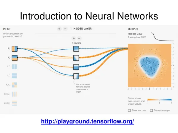
Pattern Recognition and Machine Learning 2006. Introduction to Neural Networks. Debrup Chakraborty. To be covered today. Introduction Perceptron Algorithm Multilayered Perceptrons. HAYKIN , S., "Neural Networks: A Comprehensive Foundation," Prentice Hall, Upper Saddle River, NJ, 1999.

E N D
Pattern Recognition and Machine Learning 2006 Introduction to Neural Networks Debrup Chakraborty
To be covered today Introduction Perceptron Algorithm Multilayered Perceptrons HAYKIN , S., "Neural Networks: A Comprehensive Foundation," Prentice Hall, Upper Saddle River, NJ, 1999
The Biological Neuron The human brain is made of about 100 billions of such neurons.
Characteristics of Biological Neural Networks • Massive connectivity • Nonlinear, Parallel, Robust and Fault Tolerant • Capability to adapt to surroundings • Ability to learn and generalize from known examples • Collective behavior is different from individual behavior Artificial Neural Networks mimics some of the properties of the biological neural networks
Some Properties of Artificial Neural Networks Assembly of simple processors Information stored in connections – No Memory Massively Parallel Massive connectivity Fault Tolerant Learning and Generalization Ability Robust Individual dynamics different from group dynamics All these properties may not be present in a particular network
Network Characteristics • Neural Network Characterized by: • Architecture • Learning (update scheme of weights and/or outputs) Architecture Layered (single /multiple): Feed forward – MLP, RBF Recurrent : At least one feedback loop – Hopfield Competitive : p – dimensional array of neurons with a set of nodes supplying input to each element of the array – LVQ, SOFM
Learning • Supervised : In Presence of a teacher • Unsupervised or Self-Organized : No teacher • Reinforcement: Trial and error, no teacher, but can asses the situations – reinforcement signals.
Model of an Artificial Neuron uT = (u1,u2,…,uN) The input vector wT =(w1,w2,…,wN) The weight vector
Activation Functions • Threshold Functionf(v) = 1 if v 0 = 0 otherwise • Piecewise-Linear Functionf(v) = 1 if v ½ = v if ½> v > - ½ = 0 otherwise • Sigmoid Functionf(v) = 1/{1 + exp(- av)}etc..
Perceptron Learning Algorithm Assume we are given a data set X={(x1,y1),....,( xl,yl)}, where xRn and y = {1,-1}. Assume X is linearly separable i.e.: There exists a w and b, such that (wTxi + b)yi > 0, for all i Classification of X means finding a w and b such that (wTxi + b)yi > 0, for all i A perceptron can classify X in a finite number of steps
Linearly separable OR, AND and NOT are linearly separable Boolean Functions XOR is not linearly separable
Perceptron Learning Algorithm (Contd.) f(neti) = 1 if neti > 0 f(neti) = -1 otherwise neti = wTxi Starting with w(0)=0 we follow the following learning rule: w(t+1) = w (t) +αyixi for each misclassified point xi
The Multilayered Perceptron MLPs are layered feed-forward networks. The n-th layer is fully connected with the (n+1)-th layer. They are widely used for learning input-output mappings from data which has varied scientific and engineering applications. Each node in an MLP behaves like a perceptron with a sigmoidal activation function.
Multilayered Perceptrons (Contd.) An MLP can learn efficiently any input-output mapping. Suppose we have a training set X={(x1,y1),....,( xn,yn)}, where xRp and yRq. There is an unknown functional relationship between x and y. Say, y = F(x). Our objective is to learn F, given X.
Multilayered Perceptrons (Contd.) When an input vector is given to an MLP it computes a function. The function F* which the MLP computes has the weights and biases of each nodes as a parameter. Let W be a vector which contains all the weights and biases associated with the MPL as its elements, thus the MLP computes the function F*(W,x). Our objective would be to find such a W which minimizes E = ½ i||F*(W,xi) – yi||2
The Gradient descent algorithm • Let w = ( w1,…,wN)T be a vector of N adjustable parameters. • Let J(w) be a scalar cost function, with the following properties : • Smoothness: The cost function J(w) is twice differentiable with respect to any pair (wj,wj) for 1 i j N. • Existence of Solution: At least one parameter vectorwopt = ( w1,opt,…,wN,opt)T exists, such that • a) b) The NN Hessian Matrix H(w) with entries hij(w) Is positive definite for w = wopt
The Gradient Descent Algorithm (Contd.) The minimizer for J can be found as Where w(0) is any initial parameter vector and (k) is a positive values sequence of step sizes. This optimization procedure may lead to a local minima of the cost function J.
Training the MLP The weights of a MLP which minimizes the error E can also be found by the gradient descent algorithm. This method when applied to a MLP is called the backpropagation which have two passes. Forward pass: where the output is calculated Backward pass: According to the error the weights are updated Modes of update: Batch Update Online Update
Multilayered Perceptron (Contd.) Some important issues: How big should be my network ? No specific answer is known till date. The size of the network depends on the complexity of the problem at hand and the training accuracy which is desired. A good training accuracy does not always means a good network. If the number of free parameters of the network is almost the same as the number of data points, the network tends to memorize the data and gives bad generalization. How many hidden layers to use ? It has been proved that a single hidden layer is sufficient to do any mapping task. But still experience shows that multiple hidden layers may be sometimes simplify learning.
Can a trained network generalize on all data points ? No, it can generalize only on data points which lies within the boundary of the training sample. The output given by an MLP is never reliable on data points far away from the training sample. Can I get the explicit functional form of the relationship that exists in my data from the trained MLP? No, one may write a functional form of nested sigmoids, but it will (in almost all cases) be far from useful. MLPs are black-boxes, one cannot retrieve the rules which governs the input-output mapping from a trained MLP by any easy means.
More on Generalization • A network is said to generalize well if it produces correct output (or nearly so) for a input data point never used to train the network. • The training of an MLP may be viewed as a “curve fitting” problem. The network performs useful generalization (interpolation) as MLPs with continuous activation functions leads to continuous outputs. • If an MLP have too many free parameters compared to the diversity in the data, the network may tend to memorize the training data. • Generalization ability depends on: • Representativeness of the training set • The architecture of the network • The complexity of the problem
Some applications • Function approximation • Classification a) Land Cover classification for remotely sensed images b) Optical Character Recognition many more !! • Dimensionality Reduction
Function approximation S x y The system S can be any type of system with numerical input and output.
Classification Classifiers are functions of special types which do not have numerical outputs but have class labels as outputs. D: RpNpc The class labels can be numerically coded and thus an MLP may be used to learn a classification problem. Example: We may code three different classes as 0 0 1 -- Class1 0 1 0 -- Class2 1 0 0 – Class3
Dimensionality Reduction by MLP Both the input and output nodes contains p nodes and the hidden layer contain q nodes. Here q<p. A pattern x = (x1,...,xp) is presented to the network with the same target x. If the output from the hidden layer of the trained network is tapped, then we get a transformed set of feature vectors yRq But, these feature vectors y are not interpretable. There can be other approaches too !!
Online Feature Selection by MLP Associate with each input node i a multiplier fi. fi takes values in [0,1]. fi 's takes values near one for good features and near zero for bad/redundant ones. A good choice fi = f(i) =1/(1+e-i) i's are learnable. Initialization.