Download
1 / 27
280 likes | 571 Views
Introduction to Neural Networks. http://playground.tensorflow.org/. Outline. Perceptrons Perceptron update rule Multi-layer neural networks Training method Best practices for training classifiers After that: convolutional neural networks. Recall: “Shallow” recognition pipeline.

E N D
Introduction to Neural Networks http://playground.tensorflow.org/
Outline • Perceptrons • Perceptron update rule • Multi-layer neural networks • Training method • Best practices for training classifiers • After that: convolutional neural networks
Recall: “Shallow” recognition pipeline Feature representation Trainableclassifier Image Pixels Class label • Hand-crafted feature representation • Off-the-shelf trainable classifier
“Deep” recognition pipeline • Learn a feature hierarchy from pixels to classifier • Each layer extracts features from the output of previous layer • Train all layers jointly Layer 1 Layer 2 Layer 3 Image pixels Simple Classifier
Neural networks vs. SVMs (a.k.a. “deep” vs. “shallow” learning)
Linear classifiers revisited: Perceptron Input Weights x1 w1 x2 w2 Output:sgn(wx + b) x3 w3 . . . Can incorporate bias as component of the weight vector by always including a feature with value set to 1 wD xD
Perceptron training algorithm • Initialize weights w randomly • Cycle through training examples in multiple passes (epochs) • For each training example x with label y: • Classify with current weights: • If classified incorrectly, update weights:(α is a positive learning rate that decays over time)
Perceptron update rule • The raw response of the classifier changes to • If y = 1 and y’ = -1, the response is initially negative and will be increased • If y = -1 and y’ = 1, the response is initially positive and will be decreased
Convergence of perceptron update rule • Linearly separable data: converges to a perfect solution • Non-separable data: converges to a minimum-error solution assuming examples are presented in random sequence and learning rate decays as O(1/t) where t is the number of epochs
Multi-layer perceptrons • To make nonlinear classifiers out of perceptrons, build a multi-layer neural network! • This requires each perceptron to have a nonlinearity
Multi-layer perceptrons • To make nonlinear classifiers out of perceptrons, build a multi-layer neural network! • This requires each perceptron to have a nonlinearity • To be trainable, the nonlinearity should be differentiable Sigmoid: Rectified linear unit (ReLU): g(t) = max(0,t)
Training of multi-layer networks • Find network weights to minimize the prediction loss between true and estimated labels of training examples: • Possible losses (for binary problems): • Quadratic loss: • Log likelihood loss: • Hinge loss:
Training of multi-layer networks • Find network weights to minimize the prediction loss between true and estimated labels of training examples: • Update weights by gradient descent: w2 w1
Training of multi-layer networks • Find network weights to minimize the prediction loss between true and estimated labels of training examples: • Update weights by gradient descent: • Back-propagation: gradients are computed in the direction from output to input layers and combined using chain rule • Stochastic gradient descent: compute the weight update w.r.t. one training example (or a small batch of examples) at a time, cycle through training examples in random order in multiple epochs
Network with a single hidden layer • Neural networks with at least one hidden layer are universal function approximators
Network with a single hidden layer • Hidden layer size and network capacity: Source: http://cs231n.github.io/neural-networks-1/
Regularization • It is common to add a penalty (e.g., quadratic) on weight magnitudes to the objective function: • Quadratic penalty encourages network to use all of its inputs “a little” rather than a few inputs “a lot” Source: http://cs231n.github.io/neural-networks-1/
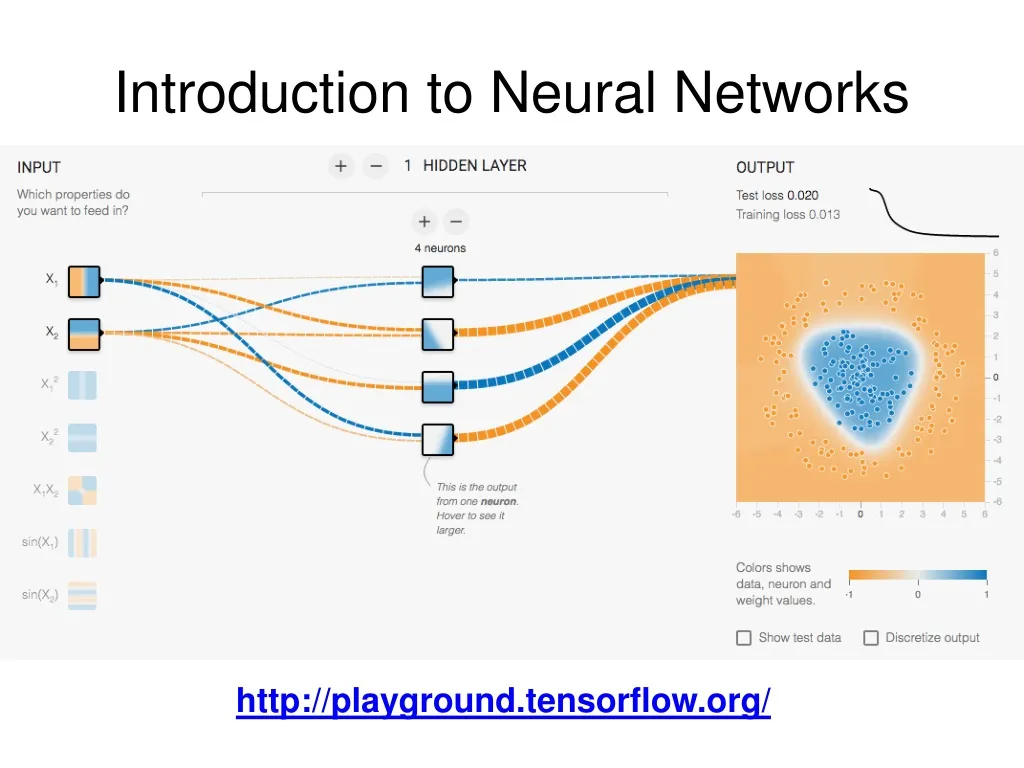
Multi-Layer Network Demo http://playground.tensorflow.org/
Dealing with multiple classes • If we need to classify inputs into C different classes, we put C units in the last layer to produce C one-vs.-others scores • Apply softmax function to convert these scores to probabilities: • If one of the inputs is much larger than the others, then the corresponding softmax value will be close to 1 and others will be close to 0 • Use log likelihood (cross-entropy) loss:
Neural networks: Pros and cons • Pros • Flexible and general function approximation framework • Can build extremely powerful models by adding more layers • Cons • Hard to analyze theoretically (e.g., training is prone to local optima) • Huge amount of training data, computing power may be required to get good performance • The space of implementation choices is huge (network architectures, parameters)
Best practices for training classifiers • Goal: obtain a classifier with good generalization or performance on never before seen data • Learn parameters on the training set • Tune hyperparameters (implementation choices) on the held out validation set • Evaluate performance on the test set • Crucial: do not peek at the test set when iterating steps 1 and 2!
http://www.image-net.org/challenges/LSVRC/announcement-June-2-2015http://www.image-net.org/challenges/LSVRC/announcement-June-2-2015
Bias-variance tradeoff • Prediction error of learning algorithms has two main components: • Bias: error due to simplifying model assumptions • Variance: error due to randomness of training set • Bias-variance tradeoff can be controlled by turning “knobs” that determine model complexity High bias, low variance Low bias, high variance Figure source
Underfitting and overfitting • Underfitting: training and test error are both high • Model does an equally poor job on the training and the test set • The model is too “simple” to represent the data or the model is not trained well • Overfitting: Training error is low but test error is high • Model fits irrelevant characteristics (noise) in the training data • Model is too complex or amount of training data is insufficient Underfitting Good tradeoff Overfitting Figure source