Download
1 / 45
460 likes | 534 Views
Introduction to Neural Networks. John Paxton Montana State University Summer 2003. Chapter 4: Competition. Force a decision (yes, no, maybe) to be made. Winner take all is a common approach. Kohonen learning w j (new) = w j (old) + a (x – w j (old))

E N D
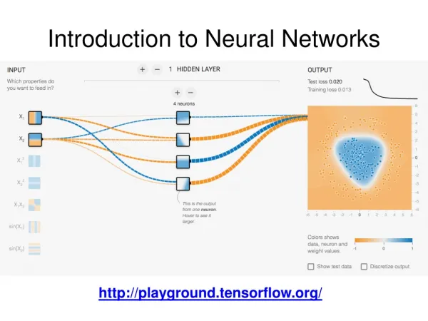
Introduction to Neural Networks John Paxton Montana State University Summer 2003
Chapter 4: Competition • Force a decision (yes, no, maybe) to be made. • Winner take all is a common approach. • Kohonen learning wj(new) = wj(old) + a (x – wj(old)) • wj is closest weight vector, determined by Euclidean distance.
MaxNet • Lippman, 1987 • Fixed-weight competitive net. • Activation function f(x) = x if x > 0, else 0. • Architecture a1 a2 1 -e 1
Algorithm 1. wij = 1 if i = j, otherwise –e 2. aj(0) = si, t = 0. 3. aj(t+1) = f[aj(t) –e*S k<>j ak(t)] 4. go to step 3 if more than one node has a non-zero activation Special Case: More than one node has the same maximum activation.
Example • s1 = .5, s2 = .1, e = .1 • a1(0) = .5, a2(0) = .1 • a1(1) = .49, a2(1) = .05 • a1(2) = .485, a2(2) = .001 • a1(3) = .4849, a2(3) = 0
Mexican Hat • Kohonen, 1989 • Contrast enhancement • Architecture (w0, w1, w2, w3) • w0 (xi -> xi) , w1 (xi+1 -> xi and xi-1 ->xi) xi-3 xi-2 xi-1 xi xi+1 xi+2 xi+3 0 - + + + - 0
Algorithm 1. initialize weights 2. xi(0) = si 3. for some number of steps do 4. xi(t+1) = f [ Swkxi+k(t) ] 5. xi(t+1) = max(0, xi(t))
Example • x1, x2, x3, x4, x5 • radius 0 weight = 1 • radius 1 weight = 1 • radius 2 weight = -.5 • all other radii weights = 0 • s = (0 .5 1 .5 0) • f(x) = 0 if x < 0, x if 0 <= x <= 2, 2 otherwise
Example • x(0) = (0 .5 1 .5 1) • x1(1) = 1(0) + 1(.5) -.5(1) = 0 • x2(1) = 1(0) + 1(.5) + 1(1) -.5(.5) = 1.25 • x3(1) = -.5(0) + 1(.5) + 1(1) + 1(.5) - .5(0) = 2.0 • x4(1) = 1.25 • x5(1) = 0
Why the name? • Plot x(0) vs. x(1) 2 1 0 x1 x2 x3 x4 x5
Hamming Net • Lippman, 1987 • Maximum likelihood classifier • The similarity of 2 vectors is taken to be n – H(v1, v2) where H is the Hamming distance • Uses MaxNet with similarity metric
Architecture • Concrete example: x1 y1 x2 MaxNet y2 x3
Algorithm 1. wij = si(j)/2 2. n is the dimensionality of a vector 3. yin.j = S xiwij + (n/2) 4. select max(yin.j) using MaxNet
Example • Training examples: (1 1 1), (-1 -1 -1) • n = 3 • yin.1 = 1(.5) + 1(.5) + 1(.5) + 1.5 = 3 • yin.2 = 1(-.5) + 1(-.5) + 1(-.5) + 1.5 = 0 • These last 2 quantities represent the Hamming distance • They are then fed into MaxNet.
Kohonen Self-Organizing Maps • Kohonen, 1989 • Maps inputs onto one of m clusters • Human brains seem to be able to self organize.
Architecture x1 y1 ym xn
Neighborhoods • Linear 3 2 1 # 1 2 3 • Rectangular 2 2 2 2 2 2 1 1 1 2 2 1 # 1 2 2 1 1 1 2 2 2 2 2 2
Algorithm 1. initialize wij 2. select topology of yi 3. select learning rate parameters 4. while stopping criteria not reached 5. for each input vector do 6. compute D(j) = S(wij – xi)2 for each j
Algorithm. 7. select minimum D(j) 8. update neighborhood units wij(new) = wij(old) + a[xi – wij(old)] 9. update a 10. reduce radius of neighborhood at specified times
Example • Place (1 1 0 0), (0 0 0 1), (1 0 0 0), (0 0 1 1) into two clusters • a(0) = .6 • a(t+1) = .5 * a(t) • random initial weights .2 .8 .6 .4 .5 .7 .9 .3
Example • Present (1 1 0 0) • D(1) = (.2 – 1)2 + (.6 – 1)2 + (.5 – 0)2 + (.9 – 0)2 = 1.86 • D(2) = .98 • D(2) wins!
Example • wi2(new) = wi2(old) + .6[xi – wi2(old)].2 .92 (bigger).6 .76 (bigger).5 .28 (smaller).9 .12 (smaller) • This example assumes no neighborhood
Example • After many epochs0 1 (1 1 0 0) -> category 20 .5 (0 0 0 1) -> category 1.5 0 (1 0 0 0) -> category 21 0 (0 0 1 1) -> category 1
Applications • Grouping characters • Travelling Salesperson Problem • Cluster units can be represented graphically by weight vectors • Linear neighborhoods can be used with the first and last cluster units connected
Learning Vector Quantization • Kohonen, 1989 • Supervised learning • There can be several output units per class
Architecture • Like Kohonen nets, but no topology for output units • Each yi represents a known class x1 y1 ym xn
Algorithm 1. Initialize the weights (first m training examples, random) 2. choose a 3. while stopping criteria not reached do (number of iterations, a is very small) 4. for each training vector do
Algorithm 5. find minimum || x – wj || 6. if minimum is target class wj(new) = wj(old) + a[x – wj(old)] else wj(new) = wj(old) – a[x – wj(old)] 7. reduce a
Example • (1 1 -1 -1) belongs to category 1 • (-1 -1 -1 1) belongs to category 2 • (-1 -1 1 1) belongs to category 2 • (1 -1 -1 -1) belongs to category 1 • (-1 1 1 -1) belongs to category 2 • 2 output units, y1 represents category 1 and y2 represents category 2
Example • Initial weights (where did these come from? 1 -1 1 -1 -1 -1 -1 1 • a = .1
Example • Present training example 3, (-1 -1 1 1). It belongs to category 2. • D(1) = 16 = (1 + 1)2 + (1 + 1)2 + (-1 -1)2 + (-1-1)2 • D(2) = 4 • Category 2 wins. That is correct!
Example • w2(new) = (-1 -1 -1 1) + .1[(-1 -1 1 1) - (-1 -1 -1 1)] =(-1 -1 -.8 1)
Issues • How many yi should be used? • How should we choose the class that each yi should represent? • LVQ2, LVQ3 are enhancements to LVQ that modify the runner-up sometimes
Counterpropagation • Hecht-Nielsen, 1987 • There are input, output, and clustering layers • Can be used to compress data • Can be used to approximate functions • Can be used to associate patterns
Stages • Stage 1: Cluster input vectors • Stage 2: Adapt weights from cluster units to output units
Stage 1 Architecture w11 v11 x1 z1 y1 xn zp ym
Stage 2 Architecture y*1 x*1 tj1 vj1 zj x*n y*m
Full Counterpropagation • Stage 1 Algorithm 1. initialize weights, a, b 2. while stopping criteria is false do 3. for each training vector pair do 4. minimize ||x – wj|| + ||y – vj|| wj(new) = wj(old) + a[x – wj(old)] vj(new) = vj(old) + b[y-vj(old)] 5. reduce a, b
Stage 2 Algorithm 1. while stopping criteria is false 2. for each training vector pair do 3. perform step 4 above 4. tj(new) = tj(old) + a[x – tj(old)] vj(new) = vj(old) + b[y – vj(old)]
Partial Example • Approximate y = 1/x [0.1, 10.0] • 1 x unit • 1 y unit • 10 z units • 1 x* unit • 1 y* unit
Partial Example • v11 = .11, w11 = 9.0 • v12 = .14, w12 = 7.0 • … • v10,1 = 9.0, w10,1 = .11 • test .12, predict 9.0. • In this example, the output weights will converge to the cluster weights.
Forward Only Counterpropagation • Sometimes the function y = f(x) is not invertible. • Architecture (only 1 z unit active) x1 z1 y1 xn zp ym
Stage 1 Algorithm 1. initialize weights, a (.1), b (.6) 2. while stopping criteria is false do 3. for each input vector do 4. find minimum || x – w|| w(new) = w(old) + a[x – w(old)] 5. reduce a
Stage 2 Algorithm 1. while stopping criteria is false do 2. for each training vector pair do 3. find minimum || x – w || w(new) = w(old) + a[x – w(old)] v(new) = v(old) + b[y – v(old)] 4. reduce b Note: interpolation is possible.
Example • y = f(x) over [0.1, 10.0] • 10 zi units • After phase 1, zi = 0.5, 1.5, …, 9.5. • After phase 2, zi = 5.5, 0.75, …, 0.1