Download
1 / 56
580 likes | 1.21k Views
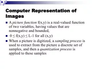
Computer Representation of Images A picture function f(x,y) is a real-valued function of two variables, having values that are nonnegative and bounded, 0 ≤ f(x,y) ≤ L-1 for all (x,y)

E N D
Computer Representation of Images • A picture function f(x,y) is a real-valued function of two variables, having values that are nonnegative and bounded, • 0 ≤ f(x,y) ≤ L-1 for all (x,y) • When a picture is digitized, a sampling process is used to extract from the picture a discrete set of samples, and then a quantization process is applied to these samples
Computer Representation of Images • The resultant digital picture function f, or digital picture, can be represented by a two-dimensional array of picture elements, or pixels • The digital picture function f can be regarded as a mapping from {0, ... , M-1}X{0, ... , N-1} to {0, ... , L-1} • The set {0, ... , L-1} is called the gray level set, and L is the number of distinct gray levels • For example, if we use 3 bits to represent each pixel, then L is 8 • If 8 bits are used, L is 256.
Computer Representation of Images • Picture Elements: Pixel • Color, • gray-value images and • binary images (e.g., values 1 for black, 0 for white) • Example • gray-value images contain different number of brightness levels:
Computer Representation of Images • M and N represent the size of the digital picture and are determined by the coarseness of the sampling • If the sampling interval is too large, the process by which a digital image was produced may be apparent to human viewers • This is the problem of undersampling • A digital image may be generated by a scanner, digital camera, frame grabber, etc.
1-bit Images • Each pixel is stored as a single bit (0 or 1), so also referred to as a binary image. • Such an image is also called a 1-bit monochrome image since it contains no color. • Fig. 3.1 shows a 1-bit monochrome image (called “Lena” by multimedia scientists - this is a standard image used to illustrate many algorithms).
Raster Display of Digital Images • The special-purpose high-speed memory for storing the image frames is called the frame buffer • The frame buffer is considered a component of the video card which are used to drive displays on modern bit-mapped displays
Bit-map Terminals • Bit-map terminals are typically used to support displays containing several windows. • Bit-map terminals require a considerable amount of video RAM. The most common sizes are 640x480 (VGA), 800x600 (SVGA), 1024x768 (XVGA), and 1280x960. Each of these has an aspect ratio of 4:3. • To get true color, 8 bits are needed for each of the three primary colors, or 3 bytes/pixel. Thus, 1024x768 requires 2.3 MB of video RAM.
Bit-map Terminals • To lessen this requirement, some computers use an 8-bit number to indicate the desired color. This number is then used as an index into a hardware table called the color palette that contains 256 entries, each holding a 24-bit RGB value. This is called indexed color. It reduces the required RAM by 2/3, but allows only 256 colors. • Usually each window on the screen has its own mapping. The palette is changed when a new window gains focus.
Bit-map Terminals • To display full-screen full-color multimedia on a 1024x768 display requires copying 2.3 MB of data to the video RAM for every frame. For full-motion video, 25 frame/sec is needed for a total data rate of 57.6 MB/sec. • This is too much for an (E)ISA bus, so high-performance video cards need to be PCI cards (or AGP)
Dithering • When an image is printed, the basic strategy of dithering is used, which trades intensity resolution for spatial resolution to provide ability to print multi-level images on 2-level (1-bit) printers. • Dithering is used to calculate patterns of dots such that values from 0 to 255 correspond to patterns that are more and more filled at darker pixel values, for printing on a 1-bit printer.
Dithering • The main strategy is to replace a pixel value by a larger pattern, say 22 or 44, such that the number of printed dots approximates the varying-sized disks of ink used in analog, in halftone printing (e.g., for newspaper photos). • 1. Half-tone printing is an analog process that uses smaller or larger filled circles of black ink to represent shading, for newspaper printing. • 2. For example, if we use a 22 dither matrix
Dithering • We can first re-map image values in 0..255 into the new range 0..4 by (integer) dividing by 256=5. Then, e.g., if the pixel value is 0 we print nothing, in a 22 area of printer output. But if the pixel value is 4 we print all four dots. • The rule is: • If the intensity is > the dither matrix entry then print an on dot at that entry location: replace each pixel by an n n matrix of dots. • Note that the image size may be much larger, for a dithered image, since replacing each pixel by a 44 array of dots, makes an image 16 times as large.
Dithering • A clever trick can get around this problem. Suppose we wish to use a larger, 44 dither matrix, such as
Dithering • An ordered dither consists of turning on the printer output bit for a pixel if the intensity level is greater than the particular matrix element just at that pixel position. • Fig. 3.4 (a) shows a grayscale image of “Lena”. The ordered-dither version is shown as Fig. 3.4 (b), with a detail of Lena's right eye in Fig. 3.4 (c).
Picture Operations • Digital images are transformed by means of one or more picture operations • An operation transforms an image I into I’ • An operation can be classified as a local operation if I’(x,y) depends only on the values of some neighborhood of the pixel (x,y) in I • If I’(x,y) depends only on the value I(x,y), then the operation is called a point operation • Operations for which the value of I’(x,y) depends on all of the pixels of I are called global operations
Picture Operations • An example of a local operation is an averaging operator which has the effect of blurring an image • The new image I’ is found by replacing each pixel (x,y) in I by the average of (x,y) and (for example) the 8 neighbors of (x,y) • Pixels on the edge of the image require special consideration
Picture Operations • The gradient operation has the opposite effect - it sharpens a picture, emphasizing edges • The gradient operator (and other local operators) can be illustrated by a template • Imagine placing the center of the template on a given pixel (x,y) in I • To compute (x,y) in I’, multiply each neighbor by the corresponding value in the template and divide by the number of pixels in the template
Picture Operations • Prewitt Operator: • -1 0 1 1 1 1 • -1 0 1 or 0 0 0 • -1 0 1 -1 -1 -1 • Sobel Operator: • -1 0 1 1 2 1 • -2 0 2 or 0 0 0 • -1 0 1 -1 -2 -1
Thresholding • Thresholding is an example of a point operation • Given a pixel value, we set the value of (x,y) in I’ to L-1 if (x,y) in I is greater than or equal to the threshold and to 0 if (x,y) is less than the threshold • The resulting image has only two values and is thus a binary image • For example, given a threshold value of 200 the image of the previous figure becomes the following
Global Operations • Nonlocal operations are called global operations • Examples include barrel distortion correction, perspective distortion correction and rotation • Camera optics may cause barrel distortion. We can correct the distortion if we know a few control points
Barrel Distortion • The mappings for barrel distortion are: • x’ = a1x + b1y + c1xy + d1 • y’ = a2x + b2y + c2xy + d2 • If we know four control points, we can solve for a1, b1 c1, d1, and a2, b2, c2, d2
Contrast Enhancement • Contrast generally refers to a difference in grayscale values in some particular region of an image function • Enhancing the contrast may increase the utility of the image. • Suppose we have a digital image for which the contrast values do not fill the available contrast range. Suppose our data cover a range (m,M), but that the available range is (n,N). Then the following linear transformation expands the values over the available range • g(x,y) = {[f(x,y)-m]/ (M-m)}[N-n]+n • This transformation may be necessary when an image has been scanned, since the image scanner may not have been adjusted to use its full dynamic range
Contrast Enhancement • For many classes of images, the “ideal” distribution of gray levels is a uniform distribution • In general, a uniform distribution of gray levels makes equal use of each quantization level and tends to enhance low-contrast information • We can enhance the contrast of an image by performing histogram equalization
Noise Removal • Noise smoothing for “snow” removal in TV images was one of the first applications of digital image processing • Certain types of “noise” are characteristic for pictures • Noise arising from an electronic sensor generally appears as random, additive errors or “snow” • In other situations, structured noise rather than random noise is persent in an image. Consider for example the scan line pattern of TV images which may be apparent to viewers
Image Data Types • The most common data types for graphics and image file formats - 24-bit color and 8-bit color. • Most image formats incorporate some variation of a compression technique due to the large storage size of image files. Compression techniques can be classified into either lossless or lossy. • In a color 24-bit image, each pixel is represented by three bytes, usually representing RGB. • Many 24-bit color images are actually stored as 32-bit images, with the extra byte of data for each pixel used to store an alpha value representing special effect information (e.g., transparency).
8-Bit Color Images • As stated before, some systems only support 8 bits of color information in producing a screen image • The idea used in 8-bit color images is to store only the index, or code value, for each pixel. Then, e.g., if a pixel stores the value 25, the meaning is to go to row 25 in a color look-up table (LUT).
How to Devise a Color Lookup Table • The most straightforward way to make 8-bit look-up color out of 24-bit color would be to divide the RGB cube into equal slices in each dimension. • The centers of each of the resulting cubes would serve as the entries in the color LUT, while simply scaling the RGB ranges 0..255 into the appropriate ranges would generate the 8-bit codes. • Since humans are more sensitive to R and G than to B, we could use 3 bits for R and G, and 2 bits for B • Can lead to edge artifacts though
How to Devise a Color Lookup Table • Median-cut algorithm: A simple alternate solution that does a better job for this color reduction problem. • (a) The idea is to sort the R byte values and find their median; then values smaller than the median are labelled with a “0” bit and values larger than the median are labelled with a “1” bit. • (b) This type of scheme will indeed concentrate bits where they most need to differentiate between high populations of close colors. • (c) One can most easily visualize finding the median by using a histogram showing counts at position 0..255. • (d) Fig. 3.11 shows a histogram of the R byte values for the forestfire.bmp image along with the median of these values, shown as a vertical line.
Popular Image File Formats • We will look at • GIF • JPEG • TIFF • EXIF • PS • PDF
GIF • GIF standard: (We examine GIF standard because it is so simple yet contains many common elements.) • Limited to 8-bit (256) color images only, which, while producing acceptable color images, is best suited for images with few distinctive colors (e.g., graphics or drawing). • GIF standard supports interlacing - successive display of pixels in widely-spaced rows by a 4-pass display process. • GIF actually comes in two flavors: • 1. GIF87a: The original specification. • 2. GIF89a: The later version. Supports simple animation via a Graphics Control Extension block in the data, provides simple control over delay time, a transparency index, etc.
GIF • Originally developed by UNISYS corporation and Compuserve for platform-independent image exchange via modem • Compression using the Lempel-Ziv-Welch algorithm (LZW) slightly modified • Localizes bit patterns which occur repeatedly • Variable bit length coding for repeated bit patterns • Well suited for image sequences (can have multiple images in a file)
GIF87 • File format overview:
GIF87 • Screen Descriptor comprises a set of attributes that belong to every image in the file. According to the GIF87 standard, it is defined as in Fig. 3.13.
GIF87 • Color Map is set up in a very simple fashion as in Fig. 3.14. However, the actual length of the table equals 2(pixel+1) as given in the Screen Descriptor.
GIF87 • Each image in the file has its own image descriptor
JPEG • JPEG: The most important current standard for image compression. • The human vision system has some specific limitations and JPEG takes advantage of these to achieve high rates of compression. • JPEG allows the user to set a desired level of quality, or compression ratio (input divided by output).