Download
1 / 20
240 likes | 573 Views
Introduction to Econometrics. Lecture 5 Extensions to the multiple regression model. Lecture plan. logarithmic transformations - log-linear (constant elasticity) models dummy variables for qualitative factors

E N D
Introduction to Econometrics Lecture 5 Extensions to the multiple regression model
Lecture plan • logarithmic transformations - log-linear (constant elasticity) models • dummy variables for qualitative factors • simple dynamic models with lagged variables - the partial adjustment mechanism • an application to illustrate the above - A study of cigarette consumption in Greece by Vasilios Stavrinos (Applied Economics, 1987 pp 323-329)
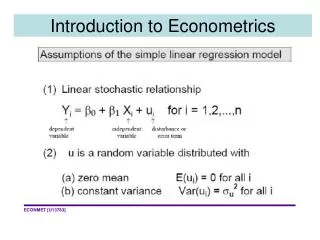
Log-linear regression models (1) In many cases relationships between economic variables may be non-linear. However we can distinguish between functional forms that are intrinsically non-linear (and will need to be estimated by some kind of iterative non-linear least squares method) and those that can be transformed into an equation to which we can apply ordinary least squares techniques.
Log-linear regression models (2) Of those non-linear equations that can be transformed, the best known is the multiplicative power function form (sometimes called the Cobb-Douglas functional form), which is transformed into a linear format by taking logarithms.
Log-linear regression models (3) Production functions For example, suppose we have cross-section data on firms in a particular industry with observations both on the output (Q) of each firm and on the inputs of labour (L) and capital (K). Consider the following functional form
Log-linear regression models (6) The parameters and can be estimated directly from a regression of the variable lnQ on lnL and lnK
Dummy variables (1) Dummy variables (sometimes called dichotomous variables) are variables that are created to allow for qualitative effects in a regression model. A dummy variable will take the value 1 or 0 according to whether or not the condition is present or absent for a particular observation. For example suppose we are investigating the relationship between the wage (Y) and the number of years of experience (X) of workers in a particular industry. Our initial model is Y = a + b X + u However we are concerned that the wages of female workers may be below that of male workers with similar experience. To test for this we can introduce a dummy variable to distinguish between the observations for male and female workers in the regression.
Dummy variables (2) Define D = 1 for male workers and 0 for female workers. The overall equation becomes Y = a + b X + cD + u where c will measure the differential between male and female workers, having taken account of differences in experience. We can run a normal multiple regression with X and D as explanatory variables. Assuming that c is positive it means that the regression line for male workers lies above that for female workers - c measures the extent of the upward shift. We can use its t value to test whether these differences are statistically significant.
Dummy variables (3) Ramu Ramanathan (1998) includes a data set compiled by Susan Wong relating to 49 professionals in an industry (23 are for females and 26 for males). The results show a large and significant difference in wages (which range between 981 and 3833 with a mean of 1820).
Dummy variables (4) Testing for differences in intercept. Yi = b1 + b2 Xi+ b3 Di+ ui Yi = (b1+ b3) + b2 Xi + ut For men:Di= 1. Y Men wage rate Women For women: Di = 0. Yi = b1 + b2 Xi + ui b1+ b3 b1 0 years of experience X
Interactive dummies: Testing for differences in intercept and slope Yi = b1 + b2 Xi + b3Di + b4Di Xi + ui Y Yi = (b1 + b3) + (b2 + b4) Xi + ui Men wage rate b2 + b4 Women Yi = b1 + b2 Xi + ui b2 b1 b1 + b3 X 0 years of experience
Dummy variables and time series data • With time series data we can have • impulsedummies – just affecting a particular period • stepdummies – affect remains on for a number of periods We might also have seasonal dummies e.g. lnQt = b0 + b1 lnYt + b2lnPt + d1D1t + d2D2t + d3 D3t + ut D1 = 1 for quarter 1 observations, 0 otherwise D2 = 1 for quarter 2 observations, 0 otherwise D3 = 1 for quarter 3 observations, 0 otherwise Beware of the “dummy variable trap”
Illustration: cigarette consumption in Greece (see Stavrinos, Applied Economics, 1987 19, pp323-329)