Download
1 / 13
170 likes | 351 Views
Partial Differential Equations. Paul Heckbert Computer Science Department Carnegie Mellon University. Differential Equation Classes 1. dimension of unknown: ordinary differential equation (ODE) – unknown is a function of one variable, e.g. y(t)

E N D
PartialDifferential Equations Paul Heckbert Computer Science Department Carnegie Mellon University 15-859B - Introduction to Scientific Computing
Differential Equation Classes 1 • dimension of unknown: • ordinary differential equation (ODE) – unknown is a function of one variable, e.g. y(t) • partial differential equation (PDE) – unknown is a function of multiple variables, e.g. u(t,x,y) • number of equations: • single differential equation, e.g. y’=y • system of differential equations (coupled), e.g. y1’=y2, y2’=-g • order • nth order DE has nth derivative, and no higher, e.g. y’’=-g 15-859B - Introduction to Scientific Computing
Differential Equation Classes 2 • linear & nonlinear: • linear differential equation: all terms linear in unknown and its derivatives • e.g. • x’’+ax’+bx+c=0 – linear • x’=t2x – linear • x’’=1/x – nonlinear 15-859B - Introduction to Scientific Computing
PDE’s in Science & Engineering 1 • Laplace’s Equation: 2u = uxx +uyy +uzz = 0 • unknown: u(x,y,z) • gravitational / electrostatic potential • Heat Equation: ut = a22u • unknown: u(t,x,y,z) • heat conduction • Wave Equation: utt = a22u • unknown: u(t,x,y,z) • wave propagation 15-859B - Introduction to Scientific Computing
PDE’s in Science & Engineering 2 • Schrödinger Wave Equation • quantum mechanics • (electron probability densities) • Navier-Stokes Equation • fluid flow (fluid velocity & pressure) 15-859B - Introduction to Scientific Computing
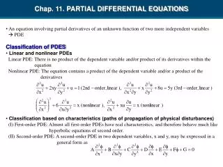
2nd Order PDE Classification • We classify conic curve ax2+bxy+cy2+dx+ey+f=0 as ellipse/parabola/hyperbola according to sign of discriminant b2-4ac. • Similarly we classify 2nd order PDE auxx+buxy+cuyy+dux+euy+fu+g=0: b2-4ac < 0 – elliptic (e.g. equilibrium) b2-4ac = 0 – parabolic (e.g. diffusion) b2-4ac > 0 – hyperbolic (e.g. wave motion) For general PDE’s, class can change from point to point 15-859B - Introduction to Scientific Computing
Example: Wave Equation • utt = c uxx for 0x1, t0 • initial cond.: u(0,x)=sin(x)+x+2, ut(0,x)=4sin(2x) • boundary cond.: u(t,0) = 2, u(t,1)=3 • c=1 • unknown: u(t,x) • simulated using Euler’s method in t • discretize unknown function: 15-859B - Introduction to Scientific Computing
k+1 k k-1 j+1 j j-1 Wave Equation: Numerical Solution u0 = ... u1 = ... for t = 2*dt:dt:endt u2(2:n) = 2*u1(2:n)-u0(2:n) +c*(dt/dx)^2*(u1(3:n+1)-2*u1(2:n)+u1(1:n-1)); u0 = u1; u1 = u2; end 15-859B - Introduction to Scientific Computing
Wave Equation Results dx=1/30 dt=.01 15-859B - Introduction to Scientific Computing
Wave Equation Results 15-859B - Introduction to Scientific Computing
Wave Equation Results 15-859B - Introduction to Scientific Computing
Poor results when dt too big dx=.05 dt=.06 Euler’s method unstable when step too large 15-859B - Introduction to Scientific Computing
PDE Solution Methods • Discretize in space, transform into system of IVP’s • Discretize in space and time, finite difference method. • Discretize in space and time, finite element method. • Latter methods yield sparse systems. • Sometimes the geometry and boundary conditions are simple (e.g. rectangular grid); • Sometimes they’re not (need mesh of triangles). 15-859B - Introduction to Scientific Computing