Download
1 / 37
880 likes | 1.95k Views
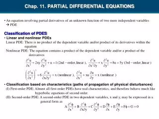
PARTIAL DIFFERENTIAL EQUATIONS. A partial differential equation is a differential equation which involves partial derivatives of one or more dependent variables with respect to one or more independent variables. Consider the first-order partial differential equation (1) In which

E N D
A partial differential equation is a differential equation which involves partial derivatives of one or more dependent variables with respect to one or more independent variables. • Consider the first-order partial differential equation (1) In which u is the dependent variable and x and y are independent variables.
The solution is; where indicates a “partial integration” with respect to “x”, holding y constant, and is an arbitrary function of y only. • Thus, solution of Eq (1) is; (2) where is an arbitrary function of y.
As a second example, consider the second-order partial differential equation: (3) • We first write this equation in the form and integrate partially with respect to y, holding x constant, where is an arbitraryfunction of x.
We now integrate this result partially with respect to x, holding y constant (4) where f defined by f(x)=is an arbitrary function of x and g is an arbitrary function of y.
The solution of the first-order partial differential equation contains one arbitrary function, and the solution of the second-order partial differential equation contains two arbitrary functions.
LINEAR PARTIAL DIFFERENTIAL EQUATIONS OF THE SECOND-ORDER The general linear partial differential equation of the second order in two independent variables x and y is; (5) where A, B, C, D, E, F and G are functions of x and y. If G(x,y)=0 for all (x,y), the Equation (5) reduces to; (6)
HOMOGENOUS LINEAR EQUATIONS OF SECOND ORDER WITH CONSTANT COEFFICIENTS (7) where a, b and c are constants. • The word homogenous refers to the fact that all terms in Equation (7) contain derivatives of the same order (the second). • u= f(y+mx) (8) where f is an arbitrary function and m is a constant. Differentiating (8);
(9) • Substituting (9) into the Equation (7); • Thus f(y+mx) will be a solution of (7) if m satisfies the quadratic equation am2+bm+c=0 (10)
we now consider the following four cases of Equation (7) • , and the roots of the quadratic Equation (10) are distinct. • ,the roots of the Equation (10) are equal.
In case (I), and the roots of Equation(10) are distinct. Let the distinct roots of Equation (10) m1 and m2. Then the Equation (7) has the solutions: f(y+m1x)+g(y+m2x)
In case (ii), , and the roots of Equation (10) are equal. Let the double root of Equation (10) be m1. The Equation (7) has the solution f(y+m1x), where f is an arbitrary function of its argument. The Equation (7) also has the solution xg(y+m1x), where g is an arbitrary function of its argument. “f(y+m1x)+ xg(y+m1x)” is a solution of Eq.7.
In case (iii), • The quadratic Equation (10) reduces to bm+c=0 and has only one root. • Denoting this root by m1, Equation (7) has the solution f(y+m1x) where f is an arbitrary function of its argument. • g(x) is an arbitrary function of x only, is also a solution of Equation (7). • f(y+m1x)+g(x) • is a solution of Equation (7).
Finally in case (iv), • The equation (10) reduces to c=0, which is impossible. • There exist no solution of the form (Equation 8). • The differential Equation (7) is; • Integrating partially with respect to y twice, we obtain • u= f(x)+ yg(x), • where f and g are arbitrary functions of x only. f(x)+yg(x) is a solution of Equation (7).
Example 1: Find a solution of (Equation 15) which contains two arbitrary functions. Solution: The quadratic Equation (10) corresponding to the differential equation (Equation 15) is; m2-5m+6=0 and this equation has the distinct roots m1=2, m2=3. Using Equation (11); u= f(y+2x)+g(y+3x) is a solution of Equation (15) which contains two arbitrary functions.
Example 2: Find a solution of (Equation 16) which contains two arbitrary functions. Solution: The quadratic Equation (14.10)corresponding to the differential equation (Equation 16) is; m2-4m+4=0 and this equation has the double root m1=2, Using Equation (12); u= f(y+2x)+xg(y+2x) is a solution of Equation (16) which contains two arbitrary functions.
The second-order linear partial differential equation (6) where A, B, C, D, E and F are real constants is said to be i) hyperbolic if B2-4AC>0 ii) parabolic if B2-4AC=0 iii) elliptic if B2-4AC<0
The equation (10) (WAVE EQUATION, a homogenous linearequation with constant coefficients) Thisequationis hyperbolic since A=1, B=0, C=-1 and B2-4AC>0. Equation (10) is a special case of the one-dimensional wave equation, which is satisfied by the small transverse displacements of the points of a vibrating string. It has the solution u=f(y+x)+g(y-x) where f and g are arbitrary functions.
The equation; (11) (HEATOR DIFFUSION EQUATION, is not homogenous) • Thisequation is parabolic, since A=1, B=C=0, andB2-4AC=0. Equation (11) is a specialcase of theone-dimensionalheatequation (ordiffusionequation), which is satisfiedbythetemperature at a point of a homogenousrod.
The equation; (12) (LAPLACE EQUATION, Homogenous linear equation with constant coefficients) • This equation is elliptic, since A=1, B=0, C=1 and B2-4AC=-4 <0. • Equation (12) is the so-called two-dimensional Laplace equation, which is satisfied by the steady-state temperature at points of a thin rectangular plate. • It has the solution; u= f (y+ix)+ g (y-ix), where f and g arearbitraryfunctions.
THE METHOD OF SEPERATION OF VARIABLES In this lesson, we introduce the so-called method of separation of variables. This is a basic method which is very powerful for obtaining solutions of certain problems involving partial differential equations. Example: Heat or Diffusion Problem We now illustrate the method of separation of variables by applying it to obtain a formal solution of the so-called heat problem.
The Physical Problem: The temperature of an infinite horizontal slab of uniform width h is everywhere zero. The temperature at the top of the slab is then set and maintained at Th, while the bottom surface is maintained at zero. Determine the temperature profile in the slab as a function of position and time.
Solution: This problem is solved in rectangular coordinates. Differential equation is; (1) The separation of variables method is now applied. We assume that the solution for T may be separated into the product of one function ψ(z) that depends solely on z, and by a second function θ(t) that depends only on t. T= T(z,t) T= ψ(z) θ(t) = ψ.θ
The left hand side of Equation (1) becomes (2) • The right hand side of Equation (1) is given by (3) • Combining equations (2) and (3) (4) where –λ2 is a constant. The boundary conditions (BC) and initial condition (IC) are now written.
BC (1) At z=0, T=0 for t ≥0 • BC (2) At z=h, T=Th for t>0 • IC At t=0, T=0 for 0≤z≤h • The following solution results if –λ2 is zero. T0=C1+C2z (5) • Substituting BC(1) and BC(2) into Equation (5) gives T0=Th (z/h) (6) The equation (6) is the steady-state solution to the partial differential equation (PDE).
If the constant is nonzero, we obtain (7) Equations (6) and (7) are both solutions to (1). Since (1) is a linear PDE, the sum of Equations (6) and (7) also is a solution, i.e., (8)
The constant an is evaluated ısing the IC. (10) Steady-state solution Transient solution
Consider the two-dimensional problem of a very thin solid bounded by the y-axis (z=0), the lines y=0 and y=l, and extending to infinity in the z direction. The temperature of the vertical edge at y=0 and y=l is maintained at zero. The temperature at z=0 is To. Determine the steady-state temperature profile in the solid. Assume both plane surfaces of the solid are insulated.
The two-dimensional view of this system is presented in the Figure. z T=0 T=0 T=To y z=0 y=0 y=L Based on the problem statement T is not a function of x. Based on the problem statement T is not a function of x.
(1) This PDE is solved using the separation-of-variables method. Since the temperature of the solid is a function of y and z, we assume the solution can be separated into the product of one function Φ (z) that depends only on z. T=T(y,z) T=ψ (y) Φ (z) (2) T=ψ Φ
The first term of Equation (1) is =Φ ψ’’ The second term makes the form = ψ Φ’’ (3) Substituting Equations (2) and (3) into Equation (1) gives Φ ψ’’+ ψ Φ’’ =0 (4) Function of y Function of z
Both terms in Equation (4) are equal to the same constant –λ2. (5) A positive constant or zero does not contribute to the solution of the problem. and are constants that depend on the value of λ. (6)
What are the BC? • BC(1) T=0 at y=0 • BC(2) T=0 at y=R • BC(3) T=To z=0 • BC(4) T=0 z=∞ Based on physical grounds, BC(4) gives, C=0
BC(1) gives bλ =0 • (7) • BC (2) gives • The RHS of this equation is zero if aλ=0 or sin λL=0. If aλis zero, no solution results. Therefore • sin λL=0 • λL=nπ; n=1,2,3,4,… • λ=( nπ)/L
The equation (7) now becomes The constant an is evaluated from BC(3). The Fourier series analysis gives So that;