Download
1 / 29
860 likes | 2.77k Views
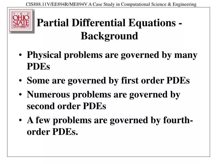
Physical problems are governed by many PDEs Some are governed by first order PDEs Numerous problems are governed by second order PDEs A few problems are governed by fourth-order PDEs. Partial Differential Equations - Background. Examples. Examples (contd.).

E N D
Physical problems are governed by many PDEs Some are governed by first order PDEs Numerous problems are governed by second order PDEs A few problems are governed by fourth-order PDEs. Partial Differential Equations - Background
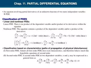
There are 6 basic classifications: (1) Order of PDE (2) Number of independent variables (3) Linearity (4) Homogeneity (5) Types of coefficients (6) Canonical forms for 2nd order PDEs Classification of Partial Differential Equations (PDEs)
The order of a PDE is the order of the highest partial derivative in the equation. Examples: (2nd order) (1st order) (3rd order) (1) Order of PDEs
Examples: (2 variables: x and t) (3 variables: r, q, and t) (2) Number of Independent Variables (3) Linearity PDEs can be linear or non-linear. A PDE is linear if the dependent variable and all its derivatives appear in a linear fashion (i.e. they are not multiplied together or squared for example.
Examples: (Linear) (Non-linear) (Linear) (Non-linear) (Non-linear) (Linear) (Non-linear)
A PDE is called homogenous if after writing the terms in order, the right hand side is zero. Examples: (Non-homogeneous) (Homogeneous) (Homogenous) (4) Homogeneity
(Non-homogeneous) (Homogeneous) Examples (5) Types of Coefficients If the coefficients in front of each term involving the dependent variable and its derivatives are independent of the variables (dependent or independent), then that PDE is one with constant coefficients.
(Variable coefficients) (C constant; constant coefficients) Examples (6) Canonical forms for 2nd order PDEs (Linear) (Standard Form) where A, B, C, D, E, F, and G are either real constants or real-valued functions of x and/or y.
PDE is Elliptic PDE is Parabolic PDE is Hyperbolic Parabolic PDE solution “propagates” or diffuses Hyperbolic PDE solution propagates as a wave Elliptic PDE equilibrium
This terminology of elliptic, parabolic, and hyperbolic, reflect the analogy between the standard form for the linear, 2nd order PDE and conic sections encountered in analytical geometry: for which when one obtains the equation for an ellipse, when one obtains the equation for a parabola, and when one gets the equation for a hyperbola.
(a) Here, A=1, B=0, C=2, D=E=F=G=0 B2-4AC = 0 - 4(1)(2) = -8 < 0 this equation is elliptic. (b) Here, A=1, B=0, C=-2, D=E=F=G=0 B2-4AC = 0 - 4(1)(-2) = 8 > 0 this equation is hyperbolic. (c) Here, A=1, B=0, E=-2, C=D=F=G=0 B2-4AC = 0 - 4(1)(0) = 0 this equation is parabolic. Examples
(d) Here, A=1, B=-4, C=1, D=E=F=G=0 B2-4AC = 16 - 4(1)(1) = 12 > 0 this equation is hyperbolic. (e) Here, A=3, B=-4, C=-5, D=E=F=G=0 B2-4AC = 16 - 4(3)(-5) = 76 > 0 this equation is hyperbolic. (f) Here, A=3, B=-4, C=-5, D=8, E=-9, F=6, G=27exy B2-4AC = 16 - 4(3)(-5) > 0 this equation is hyperbolic. Examples
(g) Here, A=y, B=0, C=-1, D=E=F=G=0 B2-4AC = 0 - 4(y)(-1) = 4y for y>0, this equation is hyperbolic; for y=0, this equation is parabolic; for y<0, this equation is elliptic. Examples
(h) Here, A=1, B=2x, C=1-y2, D=E=F=G=0 B2-4AC = 4x2 - 4(1)(1-y2) = 4x2+4y2-4 or x2+y2 >,=,< 0 Examples
(i) Here, A=1, B=-y, C=0, D=E=F=G=0 B2-4AC = y2 for y=0, this equation is parabolic; for y0, this equation is hyperbolic. Examples
(j) Here, A=sin2x, B=sin2x, C=cos2x, D=E=F=G=0 B2-4AC = sin22x-4sin2xcos2x = 4sin2xcos2x-4sin2xcos2x = 0 this equation is parabolic everywhere. Example
(k) This must be converted to 2nd order form first: and subtracting, Now, A=1, B=0, C=-1, D=E=F=G=0 B2-4AC=4 > 0 Hyperbolic. Example
(l) Again, convert to 2nd order form first: and adding, Again, A=1, B=0, C=-1, D=E=F=G=0 B2-4AC = 4 > 0 Hyperbolic. Example
The wave equation has the form: This equation can be factored as follows: This implies that x+t and x-t define characteristic directions, i.e. directions along which the PDE will collapse into an ODE. Wave equation (hyperbolic)
Let x=x+t and h=x-t Similarly, Thus, and Wave equation (contd.)
Thus, and and or, by integrating again, Wave equation (contd.)
Note that there are other important equations in mathematical physics, such as: Schroedinger eq. 1-D which is a wave equation by virtue of the imaginary constant i. Note that but for the “i” (= ), this equation would be parabolic. However, the “i” makes all the difference and this is a wave equation (hyperbolic).
We now return to the case study problem for adiabatic ( ), frictionless, quasi-1D flow: For simplicity, we have assumed that ne=0 (non-ionized flow) for now.
Recall that for steady flow, we found that M = 1 when dA/dx = 0 (choking or sonic condition), where It turns out that this system of equations exhibits elliptic character for M<1, and hyperbolic character for M>1. Thus, M=1, the choking point, exists to delineate the elliptic and hyperbolic regions of the flow.
If we are interested in transient, i.e. time-dependent solutions, analytical solutions do not exist (except for drastic simplifications) and the governing equations must be solved numerically. If we are interested in obtaining steady state solutions, they can be obtained numerically as well (in quasi-1D flow, analytical solutions were obtained), in one of two ways: Direct solution of steady state equations, or Time-marching from an arbitrary initial state to the steady state.
At steady state, An analytical solution can be obtained for this case. Conservation equations for quasi-1D, isothermal flow
A steady state solution can also be obtained by time-marching, i.e. solving the unsteady equations: Conservation equations for quasi-1D, isothermal flow (contd.)