Download
1 / 1
10 likes | 87 Views
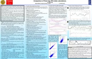
New Unifying Procedure for PC index calculations. P. Stauning Danish Meteorological Institute (e-mail: pst@dmi.dk /phone : + 45 39157473) ).

E N D
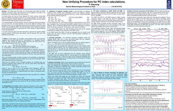
New Unifying Procedure for PC index calculations. P. Stauning Danish Meteorological Institute (e-mail: pst@dmi.dk/phone: + 45 39157473) ) 6. PC index coefficients at AARI, DTUS and DMI. The different ways to calculate magnetic variations are not the only difference between the three current PC index variants (AARI, DTU-S, and DMI). The AARI and DTU-S (=old DMI) versions include reverse convection cases in the data set used for calculation of coefficients, which is why the intercept values tend to become strongly negative during local summer days (Fig.2c below). The DMI version excludes reverse convection cases in the calculation of coefficients (not in the calculation of PC index values). Accordingly, the β-value is close to zero. The coefficients: optimum angle, slope, and intercept values derived for PCN in the three versions are displayed below. Each monthly segment (1/12 of the diagram width) displays the monthly average daily variation in the selected parameter. • Effects of reverse convection on PC indices. With the slope and intercept data presented in the above figures (Figs. 2a-c), the formula for the PC index (Eqs.3 and 4) and the approximations (Eqs. 5a and 5b), it is easy to see the effect of including/excluding reverse convection cases. • Including reverse convection cases makes the intercept more negative. Thus a positive term is added to the PC index value. The slope is increased, which reduces the PC index values. The combined effect is an increase of PC index values at low disturbance levels and a decrease of PC index values at high disturbance levels. In the example below PCN-DMIA are PCN values calculated using AARI coefficients and DMI QDC procedure. The other index values are contributed from their respective producers.: • Abstract.The Polar Cap (PC) index is a controversial topic within the IAGA scientific community. Since 1997 discussions of the validity of the index to be endorsed as an official IAGA index have ensued. • Currently, there are now the three separate PC index versions constructed from the different procedures used at the three institutes: the Arctic and Antarctic Research Institute (AARI), the Danish Meteorological Institute (DMI), and the Danish National Space Institute (DTU Space). • It is demonstrated in this presentation, that two consistent unifying procedures can be built from the best elements of the three different versions. One procedure uses a set of coefficients aimed at the calculation of final PC index values to be accepted by IAGA. The other procedure uses coefficients aimed at on-line real-time production of preliminary PC index values for Space Weather monitoring applications. • For each of the two cases the same procedure is used for the northern (PCN) and the southern (PCS) polar cap indices, and the derived PCN and PCS coefficients are similar. 3. Definition of magnetic variation vector. In the calculation of magnetic variations, three variants have developed to derive the magnetic variation vector, ΔF, from the observed magnetic data, FOBS , which could be described by the following defining equations: ΔF = FOBS - FBL …. DTU-S (formerly DMI#2) (6a) ΔF = (FOBS - FBL) - FQDC …..DMI (6b) ΔF = (FOBS - FBL– ΔFY) - FQDC .... AARI (6c) In these expressions FBL is the slowly (secularly) varying baseline vector for the day in question; FQDC is the quiet day (QDC) variation vector for the time in question; ΔFY is an IMF By-related (solar wind sector dependent) correction vector for the day in question. The terms FBL+ ΔFY could be combined. In the present DMI method the IMF By-related (solar wind sector related) contribution is included in the calculation of the QDC vector. In the AARI version the QDC is found by averaged over an interval much longer than the sector structure and the IMF By-related contribution is calculated separately. Fig.4 Fig.2a 4. Intercept parameter. For extremely quiescent conditions, where the merging electric field, Em, is zero, we would expect that the magnetic deflection shall resort to just depict the QDC variation. Hence, according to Eq. 2, the so-called intercept value, β, must be equal to ΔFPROJ , i.e., the variation vector projected to the optimum direction. If the QDC vector has already been subtracted from the total variation vector (AARI and DMI procedure), then the resulting variation is zero, and thus the intercept value, β, must also be zero. Since the β value should be zero for each case of Em=0, then the smoothing over long time should not change the result, i.e.: β = = 0. If the QDC has not been subtracted from the variation vector (DTU-S procedure), then the intercept value, β, must be equal to the projected QDC vector according to Eq. 2. Since the value of β is formed by averaging over some time (several years) then the resulting β-value should equal the average value of the projected QDC vector. 5. Reverse convection. When actual calculations give another result, then the calculations are possibly influenced by cases of reverse convection. Figs. 1a,b illustrate the consequences of reverse convection cases for the calculation of regression coefficients. We consider observations made at the same UT time on several consecutive days. For these days the projected QDC level is assumed to be Fq at the selected UT time. For the 3 days we assume that corresponding values of Em and ΔFproj are known and they are marked in the plots. The QDC value, Fq, is subtracted to provide a set of three corrected magnetic variation values. Hence, from these three days we can calculate the slope and intercept parameters, for instance, with QD correction. Now, we assume that one day is a reverse convection case (ΔFproj <0) while on the two remaining days conditions are normal forward convection cases (ΔFproj >0). It is now easy to see that including reverse convection cases makes the slope steeper (i.e., α larger) and the intercept more negative (i.e., β more negative) • 1. Basics. A high degree of correlation exists between polar cap horizontal magnetic field variations ΔF and the ”Geo-effective” (or “merging”) Electric Field, Em, that controls the global energy input from the Solar wind to the Earth’s Magnetosphere (Kan and Lee, 1979): • Em = VSW • BT • sin2(/2) (1) • BT = (BY2 + BZ2)1/2 : IMF transverse magnetic field component • = arctan(BY/BZ) : IMF polar angle with respect to the GSM Z-axis • We may increase the correlation by projecting ΔF to an “optimum” direction in a polar cap coordinate system fixed with respect to the Sun-Earth direction. The optimum direction is characterized by the angle, φ, between the equivalent horizontal transverse current and the direction to the Sun and varies with local time and season. • ΔFPROJis a scalar quantity. A further increase in the correlation is obtained by displacing the projected horizontal variation by an amount, β(intercept), which also varies with local time and season. • Hence we are looking for the correlation between the modified polar cap horizontal magnetic field variations ΔF* and the Solar Wind ”Geo-effective Electric Field” Em of the form: • ΔF* = ΔFPROJ – β = α • Em (2) • where β (e.g. in units of nT) is the baseline shift (“intercept”), while the proportionality constant α is the “slope” (e.g. in units of nT/(mV/m)). The parameters are calculated on a statistical basis from cases of measured values through an extended epoch. • From equivalence with Em the dimensionless Polar Cap Index PC is defined by: • PC == (ΔFPROJ – β)/α(3) • The PC index is a measure of the polar geomagnetic activity corrected for daily and seasonal variations but also a proxy for the geo-effective electric field Em measured in mV/m Fig.2b Fig.2c 7. Test of effects of reverse convection on intercept. Data from Thule were used to derive the PCN coefficients (angle, slope, intercept) with exactly the same calculations (QDC subtracted) except the inclussion/omission of reverse convection cases. The results for the intercept are shown below. • The new procedure: • Calculation of coefficients for final PC index (black lines in Fig.2a-c): • Remove reverse convection cases from reference data set. • Calculate QDC and correct all magnetic variation samples. • Calculate optimum angles, φ (as usual) and project all samples to optimum direction. • Set intercept parameters, β=0 (is small anyway) and calculate best slope, α values. • Calculation of final PC index values (QDC calculations needed): • Calculate QDC and correct all magnetic variation samples. • Project all samples to optimum direction using φ. • Divide QDC-corrected, projected magnetic variation samples by α. (β=0) • Calculation of coefficients for temporary PC index (for on-line applications): • Remove reverse convection samples from reference data set. • Project all samples to optimum direction using above φ angles (from final case). • Set slope, α, to above final case values and calculate best intercept, β values. • Calculation of temporary PC index values (no need to derive actual QDC): • Project all samples to optimum direction using optimum angle , φ, from final case. • Subtract intercept, β, from projected variation samples and divide result by slope, α. 2. Interpretation of α and β. Before entering a discussion of the current PC index types, a few basic statements should be made. Eq. 3 could be written: PC = ΔFproj /α – β/ α (4) In this version it is easy to see the two limiting cases: Highly disturbed conditions: PC ~ ΔFproj/α when ΔFproj is very large (5a) Very quiet conditions: PC ~ – β/ α when ΔFproj is very small (5b) With these limiting cases it is easy to arrive at a basic understanding of the physical interpretation of the two scaling coefficients. Specifically, it should be noted, that the value of the parameter α defines the PC index’ “sensitivity” to magnetic variations, while the parameter β (in combination with α) defines the PC index value at quiescent conditions where ΔFproj is very small. Fig. 1b Fig. 1a Fig. 3a Fig. 3b