Download

1 / 41
410 likes | 478 Views
Two-Way Balanced Independent Samples ANOVA. Computations. Partitioning the SS total. The total SS is divided into two sources Cells or Model SS Error SS The model is . Partitioning the SS cells. The cells SS is divided into three sources SS A , representing the main effect of factor A

E N D
Two-Way Balanced Independent Samples ANOVA Computations
Partitioning the SStotal • The total SS is divided into two sources • Cells or Model SS • Error SS • The model is
Partitioning the SScells • The cells SS is divided into three sources • SSA, representing the main effect of factor A • SSB, representing the main effect of factor B • SSAxB, representing the A x B interaction • These sources will be orthogonal if the design is balanced (equal sample sizes) • They sum to SScells • Otherwise the analysis gets rather complicated.
Gender x Smoking History • Cell n = 10, Y2 = 145,140
Computing Treatment SS Square and then sum group totals, divide by the number of scores that went into each total, then subtract the CM.
SScellsand SSerror SSerror is then SStotal minus SSCells = 26,115 ‑ 15,405 = 10,710.
SSSmoke x Gender SSinteraction = SSCellsSSGenderSSSmoke = 15,405 ‑ 9,025 ‑ 5,140 = 1,240.
Degrees of Freedom • dftotal = N - 1 • dfA = a - 1 • dfB = b - 1 • dfAxB = (a - 1)(b -1) • dferror = N - ab
Simple Main Effects of Gender SSGender, never smoked SSGender, stopped < 1m SSGender, stopped 1m ‑ 2y
Simple Main Effects of Gender SSGender, stopped 2y - 7y SSGender stopped 7y ‑ 12 y
Simple Main Effects of Gender • MS = SS / df; F = MSeffect / MSE • MSE from omnibus model = 119 on 90 df
Interaction Plot Ability to Detect the Scent Smoking History
Simple Main Effects of Smoking • SS Smoking history for men • SS Smoking history for women • Smoking history had a significant simple main effect for women, F(4, 90) = 11.97, p < .001, but not for men, F(4, 90) = 1.43, p =.23.
Multiple Comparisons Involving A Simple Main Effect • Smoking had a significant simple main effect for women. • There are 5 smoking groups. • We could make 10 pairwise comparisons. • Instead, we shall make only 4 comparisons. • We compare each group of ex-smokers with those who never smoked.
Female Ex-Smokersvs. Never Smokers • There is a special procedure to compare each treatment mean with a control group mean (Dunnett). • I’ll use a Bonferroni procedure instead. • The denominator for each t will be:
Multiple Comparisons Involving a Main Effect • Usually done only if the main effect is significant and not involved in any significant interaction. • For pedagogical purposes, I shall make pairwise comparisons among the marginal means for smoking. • Here I use Bonferroni, usually I would use REGWQ.
Bonferroni Tests, Main Effect of Smoking • c = 10, so adj. criterion = .05 / 10 = .005. • n’s are 20: 20 scores went into each mean.
Results of Bonferroni Test Means sharing a superscript do not differ from one another at the .05 level.
Eta-Squared • For the interaction, • For gender, • For smoking history,
CI.90 Eta-Squared • Compute the F that would be obtained were all other effects excluded from the model. • For gender,
Partial Eta-Squared • Value of η2 can be affected by number and magnitude of other effects in model. • For example, if our data were only from women, SSTotal would not include SSGender and SSInteraction. • This would increase η2. • Partial eta-squared estimates effect if were not other effects in the model.
Partial Eta-Squared • For the interaction, • For gender, • For smoking history,
CI.90 on Partial Eta-Squared • If you use the source table F-ratios and df with the NoncF script, it will return confidence intervals on partial eta-squared.
Omega-Squared • For the interaction, • For gender, • For smoking history,
Assumptions • Normality within each cell • Homogeneity of variance across cells
Advantages of Factorial ANOVA • Economy -- study the effects of two factors for (almost) the price of one. • Power -- removing from the error term the effects of Factor B and the interaction gives a more powerful test of Factor A. • Interaction -- see if effect of A varies across levels of B.
One-Way ANOVA Consider the partitioning of the sums of squares illustrated to the right.SSB = 15 and SSE = 85. Suppose there are two levels of B (an experimental manipulation) and a total of 20 cases.
Treatment Not Significant MSB = 15, MSE = 85/18 = 4.722. The F(1, 18) = 15/4.72 = 3.176, p = .092. Woe to us, the effect of our experimental treatment has fallen short of statistical significance.
Sex Not Included in the Model • Now suppose that the subjects here consist of both men and women and that the sexes differ on the dependent variable. • Since sex is not included in the model, variance due to sex is error variance, as is variance due to any interaction between sex and the experimental treatment.
Add Sex to the Model Let us see what happens if we include sex and the interaction in the model. SSSex = 25, SSB = 15, SSSex*B = 10, and SSE = 50. Notice that the SSE has been reduced by removing from it the effects of sex and the interaction.
Enhancement of Power The MSB is still 15, but the MSE is now 50/16 = 3.125 and the F(1, 16) = 15/3.125 = 4.80, p = .044. Notice that excluding the variance due to sex and the interaction has reduced the error variance enough that now the main effect of the experimental treatment is significant.
Footnote • Note that the confidence interval for the interaction includes zero. This is because: • If we did not remove the effect of gender and smoking history from the error term then the effect of the interaction would no longer be statistically significant (p = .32). • If we wanted the CI to be equivalent to the ANOVA F test, we would use partial 2 and we would a confidence coefficient of (1 – 2) = .90.
Presenting the Results Participants were given a test of their ability to detect the scent of a chemical thought to have pheromonal properties in humans. Each participant had been classified into one of five groups based on his or her smoking history. A 2 x 5, Gender x Smoking History, ANOVA was employed, using a .05 criterion of statistical significance and a MSE of 119 for all effects tested. There were significant main effects of gender, F(1, 90) = 75.84, p < .001, ηp2 = .46, 90% CI [.33, .55], and smoking history, F(4, 90) = 10.80, p < .001, , ηp2 = .33, 90% CI [.17, .41],as well as a significant interaction between gender and smoking history, F(4, 90) = 2.61, p = .041, ηp2 = .10, 90% CI [.002, .18]. As shown in Table 1, women were better able to detect this scent than were men, and smoking reduced ability to detect the scent, with recovery of function being greater the longer the period since the participant had last smoked.
The significant interaction was further investigated with tests of the simple main effect of smoking history. For the men, the effect of smoking history fell short of statistical significance, F(4, 90) = 1.43, p = .23. For the women, smoking history had a significant effect on ability to detect the scent, F(4, 90) = 11.97, p < .001. This significant simple main effect was followed by a set of four contrasts. Each group of female ex-smokers was compared with the group of women who had never smoked. The Bonferroni inequality was employed to cap the familywise error rate at .05 for this family of four comparisons. It was found that the women who had never smoked had a significantly better ability to detect the scent than did women who had quit smoking one month to seven years earlier, but the difference between those who never smoked and those who had stopped smoking more than seven years ago was too small to be statistically significant.
Interaction Plot Ability to Detect the Scent Smoking History