Download
1 / 11
120 likes | 309 Views
Lecture 24 Radial Basis Network (I). Outline. Interpolation Problem Formulation Radial Basis Network Type 1. RBF is a kernel function that is symmetric w. r. t. origin. Hence its variable is r that is the norm-distance from origin. Examples of RBF. What is Radial Basis Function?.

E N D
Outline • Interpolation Problem Formulation • Radial Basis Network Type 1 (C) 2001-2003 by Yu Hen Hu
RBF is a kernel function that is symmetric w. r. t. origin. Hence its variable is r that is the norm-distance from origin. Examples of RBF What is Radial Basis Function? (C) 2001-2003 by Yu Hen Hu
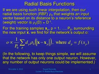
Interpolation Problem Formulation Radial Basis function for interpolation: Given {xi; 1 i K} and {di; 1 i K }, find a function F(x) that satisfies the interpolation condition: F(xi) = di 1 i K (1) One possible choice of F(x) is a radial basis function of the following form: (2) where {xi; 1 i K } are the centers of the radial basis functions. (C) 2001-2003 by Yu Hen Hu
Solving Radial Basis Coefficients • Substitute (1) into (2), we obtain a set of linear system of equations M w = d (3) where M = [M(i,j), 1 i, j, K] is the interpolation matrix, M(i,j) = (||xi – xj||), w = [w1, w2, • • •, wK]t, and d = [d1, d2, • • •, dK]t. • Given M and d, assuming the N centers are distinct, w can be solved as: w = M1d if M is non-singular. If the (r) = (r2 + c2)–1/2, or (r) = exp(–r2/(2s2)), it can further be shown that M is also positive definite. (C) 2001-2003 by Yu Hen Hu
Let F(–1) = 0.2, F(–0.5) = 0.5, and F(1) = –0.5. Use a triangular radial basis function j(r) = (1–r)[u(r) –u(r –1)] u(r) = 1 if r 0 and = 0 if r < 0. An Example (C) 2001-2003 by Yu Hen Hu rbfexample1.m
Use Gaussian rbfs: Parzen window: No weighting, and no target values of F(x) needed. , Example continued (C) 2001-2003 by Yu Hen Hu
Example (Comparison) (C) 2001-2003 by Yu Hen Hu
When there are too many data points, the M matrix may become singular. This is because by impose a rbf to each data point, we have an over-determined system. Regularization is the mathematical tool that addresses this problem. By regularization, we add an additional term to the cost function that represents additional constraints on the solution: Regularization term (e.g.): Regularization Problem Formulation (C) 2001-2003 by Yu Hen Hu
The solution to this regularization problem is G(x; xi) is the Green's function corresponding to the self-adjoin differential operator P*P such that P*P G(x; xi) = d(x – xi) A solution to the Green function that is of special interests to us is a multi-variate Gaussian function Hence With individual training data substituted into G(x, xi), a matrix equation (G + lI) w = d can be solved for w. Solution to Regularization Problem (C) 2001-2003 by Yu Hen Hu
However, other radial basis function other than the multi-variate Gaussian rbf can also be used. The regularized F(x) may no longer match data points exactly, but it will be more smooth. The value of l is usually determined empirically although generalized cross-validation (GCV) may be applied here. Implementation Consideration (C) 2001-2003 by Yu Hen Hu