Download
1 / 47
480 likes | 694 Views
Bayesian Parameter Estimation Techniques for LISA. Nelson Christensen, Carleton College, Northfield, Minnesota, USA. Outline of talk. Bayesian methods - Quick Review Fundamentals Markov chain Monte Carlo (MCMC) Methods LISA data analysis applications LISA source confusion problem

E N D
Bayesian Parameter Estimation Techniques for LISA Nelson Christensen, Carleton College, Northfield, Minnesota, USA Journées LISA-France, Meudon, May 15-16, 2006
Outline of talk • Bayesian methods - Quick Review • Fundamentals • Markov chain Monte Carlo (MCMC) Methods • LISA data analysis applications • LISA source confusion problem • Time Delay Interferometry variables • Parameter Estimation: Binary inspiral signals Journées LISA-France, Meudon, May 15-16, 2006
MCMC Collaborators • Glasgow Physics and Astronomy: Dr. Graham Woan, Dr. Martin Hendry, John Veitch • Auckland Statistics: Dr. Renate Meyer, Richard Umstätter, Christian Röver Journées LISA-France, Meudon, May 15-16, 2006
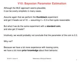
Why Bayesian methods? Orthodox statistical methods are concerned solely with deductions following experiments with populations: " The trouble is that what we [statisticians] call modern statistics was developed under strong pressure on the part of biologists. As a result, there is practically nothing done by us which is directly applicable to problems of astronomy." Jerzy Neyman, founder of frequentist hypothesis testing. Journées LISA-France, Meudon, May 15-16, 2006
Why Bayesian methods? Bayesian methods explore the joint probability space of data and hypotheses within some global model, quantifying their joint uncertainty and consistency as a scalar function: means “given” There is only one algebra consistent with this idea (and some further, very reasonable, constraints), which leads to (amongst other things) the product rule: Journées LISA-France, Meudon, May 15-16, 2006
Prior Likelihood We can usually calculate all these terms Why Bayesian methods? Bayes’ theorem: the appropriate rule for updating our degree of belief (in one of several hypotheses within some world view) when we have new data: Posterior Evidence, or “global likelihood” Journées LISA-France, Meudon, May 15-16, 2006
Marginalisation • We can also deduce the marginal probabilities. If X and Y are propositions that can take on values drawn from and then this gives us the probability of X when we don’t care about Y. In these circumstances, Y is known as a nuisance parameter. • All these relationships can be smoothly extended from discrete probabilities to probability densities, e.g.where “p(y)dy” is the probability that y lies in the range y to y+dy. =1 Journées LISA-France, Meudon, May 15-16, 2006
Markov Chain Monte Carlo methods • We need to be able to evaluate marginal integrals of the form • The approach is to sample in the space so that the density of samples reflects the posterior probability . • MCMC algorithms perform random walks in the parameter space so that the probability of being in a hypervolume dV is . • The random walk is a Markov chain: the transition probability of making a step depends on the proposed location, and the current location • MCMC - demonstrated success with problems with large parameter number. • Used by Google, WMAP, Financial Markets, LISA??? Journées LISA-France, Meudon, May 15-16, 2006
Metropolis-Hastings Algorithm • We want to explore . Let the current location be . • Choose a candidate state using a proposal distribution . • Compute the Metropolis ratio • If R>1 then make the step (i.e., )if R<1 then make the step with probability R, otherwise set , so that the location is repeated.i.e., make the step with an acceptance probability • Choose the next candidate based on the (new) current position… r Journées LISA-France, Meudon, May 15-16, 2006
Metropolis-Hastings Algorithm • {at} form a Markov chain drawn from p(a), so a histogram of {at}, or any of its components, approximates the (joint) pdf of those components. • The form of the acceptance probability guarantees reversibility even for proposal distributions that are asymmetric. • There is a burn-in period before the equilibrium distribution is reached: Journées LISA-France, Meudon, May 15-16, 2006
Application to LISA data analysis Source Confusion Problem TDI Variables Parameter Estimation for Signals Journées LISA-France, Meudon, May 15-16, 2006
LISA source identification • This has implications for the analysis of LISA data, which is expected to contain many (perhaps 50,000) signals from white dwarf binaries. The data will contain resolvable binaries and binaries that just contribute to the overall noise (either because they are faint or because their frequencies are too close together).Bayes can sort these out without having to introduce ad hoc acceptance and rejection criteria, and without needing to know the “true noise level” (whatever that means!). Journées LISA-France, Meudon, May 15-16, 2006
Things that are not generally true • “A time series of length T has a frequency resolution of 1/T.” Frequency resolution also depends on signal-to-noise ratio. We know the period of PSR 1913+16 to 1e-13 Hz, but haven’t been observing it for 3e5 years. In fact frequency resolution is • “you can subtract sources piece-wise from data.” Only true if the source signals are orthogonal over the observation period. • “frequency confusion sets a fundamental limit for low-frequency LISA.” This limit is set by parameter confusion, which includes sky location and other relevant parameters (with a precision dependent on snr). Journées LISA-France, Meudon, May 15-16, 2006
LISA source identification • Toy (zeroth-order LISA) problem: You are given a time series of 1000 data points comprising a number of sinusoids embedded in gaussian noise. Determine the number of sinusoids, their amplitudes, phases and frequencies and the standard deviation of the noise. • We could think of this as comparing hypotheses Hm that there are m sinusoids in the data, with m ranging from 0 to mmax. Equivalently, we could consider this a parameter fitting problem, with m an unknown parameter within the global model. signalparameterised bygiving dataand a likelihood Journées LISA-France, Meudon, May 15-16, 2006
LISA source identification • With suitably chosen priors on m and am we can write down the full posterior pdf of the modelBut this is (3m+2) dimensional, with m ~100 in our toy problem, so the direct evaluation of marginal pdfs for, say, m or mor to extract the pdf of a component amplitude, is unfeasible. • Explore this space using a modified Markov Chain Monte Carlo technique… Journées LISA-France, Meudon, May 15-16, 2006
Reversible Jump MCMC • Trans-dimensional moves (changing m) cannot be performed in conventional MCMC. We need to make jumps from to dimensions • Reversibility is guaranteed if the acceptance probability for an upward transition is where is the Jacobian determinant of the transformation of the old parameters [and proposal random vector r drawn from q(r)] to the new set of parameters, i.e. . • We use two sorts of trans-dimensional moves: • ‘split and merge’ involving adjacent signals • ‘birth and death’ involving single signals Journées LISA-France, Meudon, May 15-16, 2006
Trans-dimensional split-and-merge transitions • A split transition takes the parameter subvector from ak and splits it into two components of similar frequency but about half the amplitude: A A f f Journées LISA-France, Meudon, May 15-16, 2006
Trans-dimensional split-and-merge transitions • A merge transition takes two parameter subvectors and merges them to their mean: A A f f Journées LISA-France, Meudon, May 15-16, 2006
Initial values • A good initial choice of parameters greatly decreases the length of the ‘burn-in’ period to reach convergence (equilibrium). For simplicity we use a thresholded FFT: • The threshold is set low, as it is easier to destroy bad signals that to create good ones. Journées LISA-France, Meudon, May 15-16, 2006
Simulations • 1000 time samples with Gaussian noise • 100 embedded sinusoids of form • As and Bs chosen randomly in [-1 … 1] • fs chosen randomly in [0 ... 0.5] • NoisePriors • Am,Bm uniform over [-5…5] • fm uniform over [0 ... 0.5] • has a standard vague inverse- gamma prior IG( ;0.001,0.001) Journées LISA-France, Meudon, May 15-16, 2006
results teaser (spectral density) energy energy density energy density frequency Journées LISA-France, Meudon, May 15-16, 2006
results teaser (spectral density) energy energy density energy density frequency Journées LISA-France, Meudon, May 15-16, 2006
Strong, close signals A A B f f 1/T B Journées LISA-France, Meudon, May 15-16, 2006
Signal mixing • Two signals (red and green) approaching in frequency: Journées LISA-France, Meudon, May 15-16, 2006
Marginal pdfs for m and Journées LISA-France, Meudon, May 15-16, 2006
Spectral density estimates Journées LISA-France, Meudon, May 15-16, 2006
Joint energy/frequency posterior Journées LISA-France, Meudon, May 15-16, 2006
Well-separated signals (~1/T) These signals (separated by ~1 Nyquist step) can be easily distinguished and parameterized. Journées LISA-France, Meudon, May 15-16, 2006
Closely-spaced signals Signals can be distinguished, but parameter estimation in difficult. 95% contour Journées LISA-France, Meudon, May 15-16, 2006
Source Confusion: Extensions to full LISA • We have implemented an MCMC method of extracting useful information from zeroth-order LISA data under difficult conditions. • Extension to orbital Doppler/source location information should improve source identification. This code extension is currently being tested. • Extension to TDI variables is straightforward. Raw Doppler measurements could also be used, with a suitable data covariance matrix. • There is nothing special about WD-WD signals here. Similar analyses could be performed for BH mergers, EMRI sources etc… Journées LISA-France, Meudon, May 15-16, 2006
Time Delay Interferometry (TDI) variables • Principal Component Analysis (PCA) • See Romano and Woan gr-qc/0602033 • Estimate signal parameters and noise with MCMC • All information is in the likelihood • TDI variables fall right out Journées LISA-France, Meudon, May 15-16, 2006
Simple Example with Correlated Noise Data from 2 detectors s1= p + n1 + h1 s2= p + n2 + h2 Astro-signal h1=2a and h2=a n1 and n2 uncorrelated noise, p common noise; all noise zero mean <n12> = < n22> = n2 and <p2> = p2 Uncorrelated <n1n2> = <n1p> = <n2p> = 0 Likelihood p(s1,s2|a) exp[-Q/2] Q=(si-hi)C-1ij(sj-hj) C-noise covariance matrix Journées LISA-France, Meudon, May 15-16, 2006
Principal Component Analysis C- find eigenvectors, factorize likelihood p(s1,s2|a) p(s+|a)p(s-|a) s+=s1+s2 and s-=s1-s2 where p(s+|a) exp[(s+-3a)2/(8p2 + 4n2)] p(s-|a) exp[(s--a)2 /(4n2)] For LISA p2>>n2, so there is no loss of information by doing statistical inference only on the s- term - TDI. Journées LISA-France, Meudon, May 15-16, 2006
More Realistic LISA Data streams: s1= D3p2 - p1+ n1 + h1 s’1= D2p3 - p1+ n’1 + h’1 … D - delay operator MCMC- Everything is in the likelihood. Toy problem - sinusoidal gravity wave from above LISA; 3 signal parameters and 9 noise levels. 1000 data points at 1 Hz. p2>>n2 and p>>h Journées LISA-France, Meudon, May 15-16, 2006
Trace Plots Markov Chains Posterior PDFs made from these Journées LISA-France, Meudon, May 15-16, 2006
Parameter Estimation Posterior PDFs for signal parameters and noise levels. Journées LISA-France, Meudon, May 15-16, 2006
TDI Variables: Summary • TDI variables fall out of likelihood - matches well to MCMC approach • Simplify calculation for MCMC too • Incorporate LISA complexity, step by step. Realistic noise and signal terms, LISA orbit, arm length change, etc. • MCMC methods handle large parameter number; computational time grows linearly • Long-term effort to develop realistic LISA scenario, with good prospects for success Journées LISA-France, Meudon, May 15-16, 2006
Parameter Estimation for Signals • Binary Inspiral as an MCMC exercise • Numerous parameters • MCMC can provides means for estimates • Applications for other types of signals too • Demonstrated to work with a network of ground-based interferometers - extend this work to LISA Journées LISA-France, Meudon, May 15-16, 2006
Interferometer Detection • Single Detector - 5 parameters: m1, m2, effective distance dL, phase c and time tc at coalescence • Reparameterize mass: chirp mass mc and • For multi-detectors- Coherent addition of signals • Parameters for estimation: m1, m2, c, tc, actual distance d, polarization , angle of inclination of orbital plane , sky position RA and dec Journées LISA-France, Meudon, May 15-16, 2006
Amplitude Correction Work with Inspirals We have already developed an inspiral (ground based interferometer) MCMC pipeline for signals that are 3.5 Post-Newtonian (PN) in phase, 2.5 PN in the amplitude Time domain templates, then FFT into frequency domain MCMC provides parameter estimation and statistics. Future work will include spin of masses Journées LISA-France, Meudon, May 15-16, 2006
Likelihood for Inspiral Signal • Work in the frequency domain • Detector output z(t) is the sum of gravity wave signal s(t,), that depends on unknown parameters , and the noise n(t) • z(t)=s(t,)+n(t) • Noise spectral density Sn(f) Journées LISA-France, Meudon, May 15-16, 2006
Ground based example: 2 LIGO sites and Virgo. Code works, but optimization is still in progress. Journées LISA-France, Meudon, May 15-16, 2006
MCMC LISA Summary • LISA faces extremely complex data analysis challenges • MCMC methods have demonstrated record of success with large parameter number problems • MCMC for source confusion - binary background • TDI variables, signal and noise estimation • Parameter estimation: binary inspirals and other waveforms Journées LISA-France, Meudon, May 15-16, 2006
Delayed rejection • Sampling can be improved (beyond Metropolis Hastings) if a second proposal is made following, and based on, an initial rejected proposal. The initial proposal is only rejected if this second proposal is also rejected. • Acceptance probability of the second stage has to be chosen to preserve reversibility (detailed balance):acceptance probability for 1st stage:and for the 2nd stage: • Delayed Rejection Reversible Jump Markov Chain Monte Carlo method‘DRRJMCMC’ Green & Mira (2001) Biometrika 88 1035-1053. Journées LISA-France, Meudon, May 15-16, 2006
Label-switching • As set up, the posterior is invariant under signal renumbering – we have not specified what we mean by ‘signal 1’. • Break the symmetry by ordering in frequency: • Fix m at the most probable number of signals, containing n MCMC steps. • Order the nm MCMC parameter triples (A,B,f) in frequency. • Perform a rough density estimate to divide the samples into m blocks. • Perform an iterative minimum variance cluster analaysis on these blocks. • Merge clusters to get exactly m signals. • Tag the parameter triples in each cluster. f Journées LISA-France, Meudon, May 15-16, 2006
Application to the LISA confusion problem Journées LISA-France, Meudon, May 15-16, 2006