Download
1 / 44
440 likes | 467 Views
Estimating evolutionary parameters for Neisseria meningitidis. Based on the Czech MLST dataset. Testing a model of evolution: what you need. Simulation. Real Data. Starting sequence. Choose codons at random from the observed distribution of codon usage. 1. Mutational model.

E N D
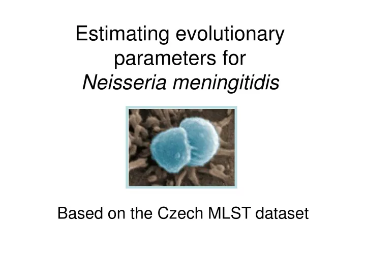
Estimating evolutionary parameters forNeisseria meningitidis Based on the Czech MLST dataset
Testing a model of evolution: what you need Simulation Real Data Starting sequence Choose codons at random from the observed distribution of codon usage 1 Mutational model Estimate evolutionary parameters from the observed data 2 Evolved sequence Statistically test for differences between simulated and observedpatterns of variation. 3 1 Codon usage frequencies 2 Mutational model of sequence evolution 3 Statistical test of hypothesis
Estimating Codon Frequency Usage Methods available: • Empirical observation of the Z2491 genome • Empirical observation of the MLST data • Bayesian inference using the MLST data
Empirical observation of the Z2491 genome Parkhill et al (2000) Complete DNA sequence of a serogroup A strain of Neisseria meningitidis Z2491. Nature404: 502-506. Nakamura et al (2000) Codon usage tabulated from the international DNA sequence databases: status for the year 2000. Nuc. Acids Res.28: 292.
Empirical observation of the MLST data Jolley et al (2000) Carried meningococci in the Czech Republic: a diverse recombining population. Journal of Clinical Microbiology38: 4492-4498
Bayesian Inference • Prior belief In the absence of any information, what might you expect codon usage to look like a priori? E.g. Codon frequency usage is unbiased and homogeneous, except for the stop codons which have zero frequency, since the sequences are coding. • Empirical data - tally the codon usage in the MLST dataset • Posterior belief Modify the prior beliefs a posteriori, following exposure to real data. The degree to which your beliefs are modified depends on the conviction with which you held your prior beliefs. The posterior beliefs will fall somewhere between the empirical observations and the prior beliefs. I.e. the posterior distribution of codon usage will be a compromise between all non-stop codons having some non-zero frequency and the observed empirical patterns of variation in codon usage.
Assumptions made in the Bayesian Inference • Refer to a triplet as a 3-base slot in the reading frame, and a codon as the specific combination of bases filling that slot. • Codon usage was modelled multinomially, i.e. each triplet is a random draw from one of the 61 possible non-stop codons. This makes the following assumptions: • The presence of one or another codon at any particular triplet is entirely independent of the codons at adjacent triplets. • All triplets are identical with respect to the probable codon usage. • We will never see any of the three STOP codons in our sequences.
Empirical observation of the MLST data Jolley et al (2000) Carried meningococci in the Czech Republic: a diverse recombining population. Journal of Clinical Microbiology38: 4492-4498
Coalescent simulations • The coalescent is a very fast way of simulating gene histories under neutral evolution. • It works because, if all mutations are neutral, then the presence/absence of mutations on the tree cannot affect its topology. • Therefore the tree topology can be simulated first, independently of the mutations. • The mutations are then superimposed onto the topology.
Mutation Selection Ancestral type Sampling usuallyoccurs at this point Neutral mutant Inviable mutant Underlying rates of non-synonymous mutation are usually confounded with selection against inviable mutants.Thus it is convenient to model functional constraint as mutational bias.(Or rather, make no attempt to disentangle the two).If we assume that the patterns of functional constraint can be modelled as a biased, but neutral, form of mutation, then we can use Coalescent simulation.
Mutational bias in Coalescent Simulations • The topology is simulated at random, as before. • As in normal coalescent simulations, mutations are superimposed onto the topology according to a Poisson process (just as in the neutral model of molecular evolution). • Those mutations, although assumed to be neutral, are biased. • The types of mutations must therefore be classified to specify the bias.
Types of single nucleotide mutationTransitions vs. transversions For any base there are always 2 possible transversions and 1 possible transition. A G Purine Transitions Transversions T C Pyramidine Transitions
T T G T T G Leucine Leucine T T A Leucine A T G Methionine Types of codon mutationSynonymous vs. non-synonymous Synonymous Non-synonymous Leucine pH 5.98 6-fold degeneracy in the genetic code Methionine pH 5.74 Single unique codon ATG CH3-S-(CH2)2-CH(NH2)-COOH (CH3)2-CH-CH2-CH(NH2)-COOH
Relative rates of the different classes of mutation m km wm wkm
Example: CTT C T T T T T A T T Leucine G T T T C T T A T T G T T T C T T A T T G
Likelihood • Having defined the model of evolution, the probability of observing different patterns in the data can be expressed. • The triplets in the MLST sequences are aligned, and the pattern of diversity in the sample at each triplet is analyzed. • The number of mutations occurring in the gene history is Poisson distributed, according to the neutral theory, with rate equal to the basic mutation rate multiplied by the evolutionary time over which mutation could have occurred. • Evolutionary time is obtained from Coalescent theory. • The basic mutation rate and the relative rates of each type of mutation are estimated from the data.
Interpreting the data in light of the model Segregating Dimorphic Segregating Dimorphic Segregating Trimorphic Non-segregating Monomorphic A T C T T G G G T G A G A T C T T G G G T G A G A T C T T G G G C G A G A T C T T G G G A G A G A T T T T G G G A G A G A T T C T A G G A G A G
Interpreting the data in light of the model Segregating Dimorphic Segregating Dimorphic Segregating Trimorphic Non-segregating Monomorphic A T C T T G G G T G A G A T C T T G G G T G A G A T C T T G G G C G A G A T C T T G G G A G A G A T T T T G G G A G A G A T T C T A G G A G A G
A A A A T T T T T C C T Interpreting the data in light of the model A T C A T C A T C A T C A T T A T T Make the assumption that no more than a single mutation occurs anywhere in the tree since the most recent common ancestor.
Interpreting the data in light of the model A T C A T C A T C A T C A T C A T T A T T Synonymous transition, rate km/M A T C Synonymous transition, rate km/M A T C A T C A T T A T C A T T A T T For a dimorphic segregating triplet, on the assumption that no more than a single mutation has occurred, ancestral type is irrelevant.
Interpreting the data in light of the model From Coalescent Theory, the evolutionary time over which mutations can occur for a gene history of n genes is given by the Watterson constant: If M is the basic rate of mutation per codon and the number of mutations in the tree is Poisson distributed, then
Interpreting the data in light of the model Segregating Dimorphic Segregating Dimorphic Segregating Trimorphic Non-segregating Monomorphic A T C T T G G G T G A G A T C T T G G G T G A G A T C T T G G G C G A G A T C T T G G G A G A G A T T T T G G G A G A G A T T C T A G G A G A G One synonymous transition inferred
Interpreting the data in light of the model Segregating Dimorphic Segregating Dimorphic Segregating Trimorphic Non-segregating Monomorphic A T C T T G G G T G A G A T C T T G G G T G A G A T C T T G G G C G A G A T C T T G G G A G A G A T T T T G G G A G A G A T T C T A G G A G A G One synonymous transition inferred One synonymous transition inferred
C T C T T T T T A G A G Interpreting the data in light of the model T T G T T G T T G T T G T T G C T A Under the assumption of no more than a single mutation this change cannot occur. Its frequency is assumed negligible, and any occurrences in the data are ignored.
Interpreting the data in light of the model Segregating Dimorphic Segregating Dimorphic Segregating Trimorphic Non-segregating Monomorphic A T C T T G G G T G A G A T C T T G G G T G A G A T C T T G G G C G A G A T C T T G G G A G A G A T T T T G G G A G A G A T T C T A G G A G A G One synonymous transition inferred One synonymous transition inferred Inference not possible, incidence assumed negligible
Interpreting the data in light of the model Segregating Dimorphic Segregating Dimorphic Segregating Trimorphic Non-segregating Monomorphic A T C T T G G G T G A G A T C T T G G G T G A G A T C T T G G G C G A G A T C T T G G G A G A G A T T T T G G G A G A G A T T C T A G G A G A G One synonymous transition inferred One synonymous transition inferred Inference not possible, incidence assumed negligible
Interpreting the data in light of the model Segregating Dimorphic Segregating Dimorphic Segregating Trimorphic Non-segregating Monomorphic A T C T T G G G T G A G A T C T T G G G T G A G A T C T T G G G C G A G A T C T T G G G A G A G A T T T T G G G A G A G A T T C T A G G A G A G One synonymous transition inferred One synonymous transition inferred Inference not possible, incidence assumed negligible Inference not possible, incidence assumed negligible
Interpreting the data in light of the model Segregating Dimorphic Segregating Dimorphic Segregating Trimorphic Non-segregating Monomorphic A T C T T G G G T G A G A T C T T G G G T G A G A T C T T G G G C G A G A T C T T G G G A G A G A T T T T G G G A G A G A T T C T A G G A G A G One synonymous transition inferred One synonymous transition inferred Inference not possible, incidence assumed negligible Inference not possible, incidence assumed negligible
G A G G A G G A G G A G G A G G A G Interpreting the data in light of the model Why might a site be monomorphic? Where x and y are the number of possible non-synonymous transversions and transitions respectively from codon GAG. Therefore
Interpreting the data in light of the model Segregating Dimorphic Segregating Dimorphic Segregating Trimorphic Non-segregating Monomorphic A T C T T G G G T G A G A T C T T G G G T G A G A T C T T G G G C G A G A T C T T G G G A G A G A T T T T G G G A G A G A T T C T A G G A G A G One synonymous transition inferred One synonymous transition inferred Inference not possible, incidence assumed negligible Inference not possible, incidence assumed negligible No mutation or inviable non-synonymous mutation
Mutation type Probability Synonymous transition Synonymous transition Non-synonymous transversion Non-synonymous transition No change Interpreting the data in light of the model
Interpreting the data in light of the model Segregating Dimorphic Segregating Dimorphic Segregating Trimorphic Non-segregating Monomorphic A T C T T G G G T G A G A T C T T G G G T G A G A T C T T G G G C G A G A T C T T G G G A G A G A T T T T G G G A G A G A T T C T A G G A G A G One synonymous transition inferred One synonymous transition inferred Inference not possible, incidence assumed negligible Inference not possible, incidence assumed negligible No mutation or inviable non-synonymous mutation Total 1094 315 27 52 700
Maximum likelihood estimation of m, k and w • It is assumed that no more than a single mutation has occurred at each triplet since the most recent common ancestor of all sequences. • This avoids inference of ancestral types. • And allows dimorphic segregating sites to be directly classified into one of the four mutation types. • However, it wastes some information: • Some triplets that are segregating cannot be classified because they involve more than a single point mutation. Rather than attempt to infer the order of mutational events, the data is ignored. • E.g. TTG and CTA both encode Leucine, but to get from one to the other requires multiple point mutations at positions 1 and 3. • If a triplet is segregating for more than a single codon (e.g. it is trimorphic) in the sample then ancestral type would need to be inferred. Rather than do that, the data is ignored. • Maximum likelihood is then used to find the most probable values of m, k and w given the observed data.
Maximum likelihood estimation of m, k and w • In maximum likelihood estimation, a formula for the probability of the data given a set of values for the parameters (m, k and w) is found. Then the values of the parameters are varied until a set are chosen for which the data is the most probable. • In this case, as there are 3 parameters, an animation is used to represent variation in kappa by a fourth dimension, time.
Maximum likelihood estimation of m, k and w • The maximum likelihood estimates were • = 0.001662 (per 2N generations) • = 5.848 • = 0.2598 • Therefore the rates, per codon per 2N generations were • Synonymous transversion 0.001662 • Synonymous transition 0.00972 • Non-synonymous transversion 0.0004318 • Non-synonymous transition 0.002525 • where N is the effective population size
Underlying mutation rate, M • Under the parameters estimated, the basic mutation rate per codon, M = 0.03819 per 2N generations, where N is the effective population size. • Biochemical estimates of the basic mutation rate in Escherichia coli have been of the order of 5 x 10⁻⁹ per generation. • Equating this to the true underlying mutation rate, the effective population size can be estimated as N = 1.3million. • Such an estimate is subject to assumptions of selective neutrality, once functional constraint has been modelled as mutational bias. • In a human pathogen such as Neisseria meningitidis, selective neutrality is highly unlikely. E. coli rate from Drake et. al. 1998 or Drake & Holland 1999
Statistical hypothesis testing • This is the next stage. • First the coalescent simulations need running. • Then we can test the MLST data for selective neutrality. • I expect neutrality to be overwhelmingly rejected as a null hypothesis. • Then we can go on to test the clonal epidemic model.