Download
1 / 16
200 likes | 801 Views
Closed-Loop Stability. Motivating example General stability criterion Routh stability criterion Direct substitution method Simulink example. Motivating Example. Transfer functions Step response for setpoint change. Motivating Example cont. Linear Stability. Linear system stability

E N D
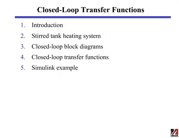
Closed-Loop Stability • Motivating example • General stability criterion • Routh stability criterion • Direct substitution method • Simulink example
Motivating Example • Transfer functions • Step response for setpoint change
Linear Stability • Linear system stability • A linear system is stable if the output response is bounded for all bounded inputs. Otherwise the system is unstable. • Open-loop stability • System that have poles with positive real part are unstable. • Integrating systems are unstable. • The closed-loop stability problem • Determine the range of controller parameter values for which the closed-loop system.
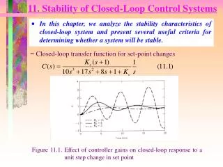
The Characteristic Equation • Closed-loop transfer function for setpoint change • Step response for distinct poles • Characteristic equation
General Linear Stability Criterion • A feedback control system is stable if and only if all the roots of the characteristic equation has negative real part.
Applying the Stability Criterion • Transfer functions • Characteristic equation • Roots
Routh Stability Criterion • Disadvantage of general stability criterion • Must explicitly compute roots in terms of controller parameters • Must deduce range of controller parameter values that produce roots with positive real parts • Routh method • Allows stable controller parameter values to be determined without explicitly calculating roots of characteristic equation • Only applicable to characteristic equations that are polynomial functions of s • Time delays must be approximated (e.g. Pade approximation)
Routh Stability Criterion cont. • Characteristic equation • Assume: an > 0 (otherwise make multiply equation by -1) • Necessary condition for stability is that all the coefficients (a0, a1,…, an-1, an) are positive • Routh array elements • Routh stability criterion: A necessary and sufficient condition for the feedback control system to be stable is for all the elements (b1, c1, …) in the left-hand column of the Routh array to be positive.
Routh Stability Criterion Example • Characteristic equation (n = 3) • Necessary condition • Elements of Routh array • Stability range: -1 < Kc < 12.6
Direct Substitution Method • Any point in the complex plane can be represented as: s = a+jw • Along the imaginary axis that divides the stable and unstable regions: s = jw • Substitute s = jw into characteristic equation to determine stability limits in terms of controller parameters • Generates two equations for real and imaginary parts of equation
Direct Substitution Example • Characteristic equation • Substitute s = jw • Separate real and imaginary parts • Stability range: -1 < Kc < 12.6
Simulink Example • Transfer functions >> gp=tf([1],[5 1]); >> gv=tf([1],[2 1]); >> gm=tf([1],[1 1]); >> gc=6; >> km=1; >> gcl=km*gc*gv*gp/(1+gc*gv*gp*gm) Transfer function: 60 s^3 + 102 s^2 + 48 s + 6 ------------------------------------------------ 100 s^5 + 240 s^4 + 209 s^3 + 143 s^2 + 57 s + 7 >>isstable(gcl) ans = 1 >> pole(gcl) ans = -1.4791 -0.1105 + 0.6790i -0.1105 - 0.6790i -0.5000 -0.2000 >> zero(gcl) ans = -1.0000 -0.5000 -0.2000
Pole-Zero Map >> pzmap(gcl)
Root Locus >> g=gp*gv*gm Transfer function: 1 ------------------------- 10 s^3 + 17 s^2 + 8 s + 1 >> rlocus(g)