Download
1 / 59
600 likes | 880 Views
Ray Tracing. CSE167: Computer Graphics Instructor: Steve Rotenberg UCSD, Fall 2005. Ray Tracing. Ray tracing is a powerful rendering technique that is the foundation of many modern photoreal rendering algorithms

E N D
Ray Tracing CSE167: Computer Graphics Instructor: Steve Rotenberg UCSD, Fall 2005
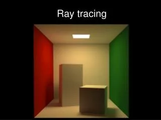
Ray Tracing • Ray tracing is a powerful rendering technique that is the foundation of many modern photoreal rendering algorithms • The original ray tracing technique was proposed in 1980 by Turner Whitted, although there were suggestions about the possibility in scientific papers dating back to 1968 • Classic ray tracing shoots virtual view rays into the scene from the camera and traces their paths as they bounce around • With ray tracing, one can achieve a wide variety of complex lighting effects, such as accurate shadows and reflections/refractions from curved surfaces • Achieving these effects with the same precision is difficult if not impossible with a more traditional rendering pipeline • Ray tracing offers a big advance in visual quality, but comes with an expensive price of notoriously slow rendering times
Ray Intersections • Tracing a single ray requires determining if that ray intersects any one of potentially millions of primitives • This is the basic problem of ray intersection • Many algorithms exist to make this not only feasible, but remarkably efficient • Tracing one ray is a complex problem and requires serious work to make it run at an acceptable speed • Of course, the big problem is the fact that one needs to trace lots of rays to generate a high quality image
Rays • Recall that a ray is a geometric entity with an origin and a direction • A ray in a 3D scene would probably use a 3D vector for the origin and a normalized 3D vector for the direction class Ray { Vector3 Origin; Vector3 Direction; };
Camera Rays • We start by ‘shooting’ rays from the camera out into the scene • We can render the pixels in any order we choose (even in random order!), but we will keep it simple and go from top to bottom, and left to right • We loop over all of the pixels and generate an initial primary ray (also called a camera ray or eye ray) • The ray origin is simply the camera’s position in world space • The direction is computed by first finding the 4 corners of a virtual image in world space, then interpolating to the correct spot, and finally computing a normalized direction from the camera position to the virtual pixel Primary ray Virtual image Camera position
Ray Intersection • The initial camera ray is then tested for intersection with the 3D scene, which contains a bunch of triangles and/or other primitives • If the ray doesn’t hit anything, then we can color the pixel to some specified ‘background’ color • Otherwise, we want to know the first thing that the ray hits (it is possible that the ray will hit several surfaces, but we only care about the closest one to the camera) • For the intersection, we need to know the position, normal, color, texture coordinate, material, and any other relevant information we can get about that exact location • If we hit somewhere in the center of a triangle, for example, then this information would get computed by interpolating the vertex data
Ray Intersection • We will assume that the results of a ray intersection test are put into some data structure which conveniently packages it together class Intersection { Vector3 Position; Vector3 Normal; Vector2 TexCoord; Material *Mtl; float Distance; // Distance from ray origin to intersection };
Lighting • Once we have the key intersection information (position, normal, color, texture coords, etc.) we can apply any lighting model we want • This can include procedural shaders, lighting computations, texture lookups, texture combining, bump mapping, and more • Many of the most interesting forms of lighting involve spawning off additional rays and tracing them recursively • The result of the lighting equation is a color, which is used to color the pixel
Shadow Rays • Shadows are an important lighting effect that can easily be computed with ray tracing • If we wish to compute the illumination with shadows for a point, we shoot an additional ray from the point to every light source • A light is only allowed to contribute to the final color if the ray doesn’t hit anything in between the point and the light source • The lighting equation we looked at earlier in the quarter can easily be adapted to handle this, as clgti will be 0 if the light is blocked • Obviously, we don’t need to shoot a shadow ray to a light source if the dot product of the normal with the light direction is negative • Also, we can put a limit of the range of a point light, so they don’t have an infinite influence (bending the laws of physics)
Shadow Rays • Shadow rays behave slightly differently from primary (and secondary) rays • Normal rays (primary & secondary) need to know the first surface hit and then compute the color reflected off of the surface • Shadow rays, however, simply need to know if something is hit or not • In other words, we don’t need to compute any additional shading for the ray and we don’t need to find the closest surface hit • This makes them a little faster than normal rays
Offsetting Spawned Rays • We say that the shadow rays are spawned off of the surface, or we might say that the primary ray spawned off additional shadow rays • When we spawn new rays from a surface, it is usually a good idea to apply a slight adjustment to the origin of the ray to push it out slightly (0.00001) along the normal of the surface • This fixes problems due to mathematical roundoff that might cause the ray to spawn from a point slightly below the surface, thus causing the spawned ray to appear to hit the same surface
Reflection Rays • Another powerful feature often associated with ray tracing is accurate reflections off of complex surfaces • If we wanted to render a surface as a perfect mirror, instead of computing the lighting through the normal equation, we just create a new reflection ray and trace it into the scene • Remember that primary rays are the initial rays shot from the camera. Any reflected rays (and others, like refracted rays, etc.), are called secondary rays • Reflected rays, like shadow rays should be moved slightly along the surface normal to prevent the ray from re-intersecting the same surface
Reflections • If the reflection ray hits a normal material, we just compute the illumination and use that for the final color • If the reflection ray hits another mirror, we just recursively generate a new reflection ray and trace that • In this way, we can render complex mirrored surfaces that include reflections, reflections of reflections, reflections of reflections of reflections… • To prevent the system from getting caught in an infinite loop, it is common to put an upper limit on the ‘depth’ of the recursion. 10 or lower works for most scenes, except possibly for ones with lots of mirrored surfaces • In any case, most pixels will only require a few bounces, as they are likely to hit a non-mirrored surface sooner or later
Reflections • Surfaces in the real world don’t act as perfect mirrors • Real mirrors will absorb a small amount of light and only reflect maybe 95%-98% of the light • Some reflecting surfaces are tinted and will reflect different wavelengths with different strengths • This can be handled by multiplying the reflected color by the mirror color at each bounce • We can also simulate partially reflective materials like polished plastic, which have a diffuse component as well as a shiny specular component • For a material like this, we would apply the normal lighting equation, including shooting shadow rays, to compute the diffuse component, then add a contribution from a reflection ray to get the final color (the diffuse and specular components should be weighted so as not to violate conservation of energy…)
Transmission Rays • Ray tracing can also be used to accurately render the light bending in transparent surfaces due to refraction • Often, this is called transmission instead of refraction. Transmission is a more general term that also includes translucency, but I think the real reason this word is preferred is because ‘reflection’ and ‘refraction’ look too similar • When a ray hits a transparent surface (like glass, or water…), we generate a new refracted ray and trace that, in a similar way as we did for reflection • We will assume that the transmitted ray will obey Snell’s law (n1sinθ1=n2sinθ2), where n1 and n2 are the index of refraction for the two materials
n d r θ1 n1 z n2 θ2 θ2 t Computing Transmission (Refraction) Direction
Total Internal Reflection • When light traveling in a material with a high index of refraction hits a material with a low index of refraction at a steep angle, we get a total internal reflection • When this happens, no refraction ray is generated • This effect can be visible when one is scuba diving and looks up at the water surface. One can only see rays refracting to the outside world in a circular area on the water surface above • Total internal reflection can be detected when the magnitude of the z vector is greater than 1, causing the square root operation to become undefined n d r θ1 n1 z n2
Spawning Multiple Rays • When light hits a transparent surface, we not only see refraction, but we get a reflection off of the surface as well • Therefore, we will actually generate two new rays and trace both of them into the scene and combine the results • The results of an individual traced ray is a color, which is the color of the light that the ray ‘sees’ • This color is used as the pixel color for primary rays, but for secondary rays, the color is combined somehow into the final pixel color • In a refraction situation, for example, we spawn off two new rays and combine them according to the Fresnel equations, provided in the last lecture • The Fresnel equations describe how the transmitted (refracted) ray will dominate when the incoming ray is normal to the surface, but the reflection will dominate when the incoming ray is edge-on
Refraction Reflection ray Camera Normal Primary ray Transmission ray
Fresnel Equations • The Fresnel equations can be used to determine the proportion of the light reflected (fr) and transmitted (ft) when a ray hits an interface between two dielectrics (like air and water) • They describe separate formulas for the parallel and perpendicularly polarized light, but these are usually averaged into a single set of values
Recursive Ray Tracing • The classic ray tracing algorithm includes features like shadows, reflection, refraction, and custom materials • A single primary ray may end up spawning many secondary and shadow rays, depending on the number of lights and the arrangement and type of materials • These rays can be thought of as forming a tree like structure
Ray-Scene Intersection • One of the key components of a ray tracer is the system that determines what surface the ray hits • A typical 3D scene may have well over 1,000,000 primitives • As usual, triangles tend to be the primitive of choice, but one advantage of a ray tracer is that one can intersect rays with more complex surfaces such as spheres, Bezier patches, displacement mapped surfaces, fractals, and more • Sometimes, complex primitives are simply tessellated into triangles in a pre-rendering phase, and then just ray traced as triangles • Alternately, it is possible to ray trace complex surfaces directly, or to use demand-based schemes that don’t tessellate an object until a ray comes nearby
Ray-Object Intersection • We will say that our scene is made up of several individual ‘objects’ • For our purposes, we will allow the concept of an object to include primitives such as triangles and spheres, or even collections of primitives or other objects • In order to be render-able, an object must provide some sort of ray intersection routine • We will define a C++ base class object as: class Object { public: virtual bool IntersectRay(Ray &r,Intersection &isect); }; • The idea is that we can derive specific objects, like triangles, spheres, etc., and then write custom ray intersection routines for them • The ray intersect routine takes a ray as input, and returns true if the object is hit and false if it is missed • If the object is hit, the intersection data is filled in into the isect class
Ray-Sphere Intersection • Let’s see how to test if a ray intersects a sphere • The ray has an origin at point p and a unit length direction u, and the sphere has a center c and a radius r c u p r
q u p c Ray-Sphere Intersection • The ray itself is the set of points p+αu, where α≥0 • We start by finding the point q which is the point on the ray-line closest to the center of the sphere • The line qc must be perpendicular to vector u, in other words, (q-c)·u=0, or (p+αu-c)·u=0 • We can solve the value of α that satisfies that relationship: α=-(p-c)·u, so q=p-((p-c)·u)u
Ray-Sphere Intersection • Once we have q, we test if it is inside the actual sphere or not, by checking if |q-c|≤r • If q is outside the sphere, then the ray must not miss • If q is inside the sphere, then we find the actual point on the sphere surface that the ray intersects • We say that the ray will hit the sphere at two points q1 and q2: q1=p+(α-a)u) q2=p+(α+a)u) where a=sqrt(r2-|q-c|2) • If α-a≥0, then the ray hits the sphere at q1, but if it is less than 0, then the actual intersection point lies behind the origin of the ray • In that case, we check if α+a≥0 to test if q2 is a legitimate intersection q2 q1 q u p c
Ray-Sphere Intersection • There are several ways to formulate the ray-sphere intersection test • This particular method is the one provided in the book • As a rule, one tries to postpone expensive operations, such as division and square roots until late in the algorithm when it is likely that there will be an intersection • Ideally, quick tests can be performed at the beginning that reject a lot of cases where the ray is far away from the object being tested
Ray-Plane Intersection • A plane is defined by a normal vector n and a distance d, which is the distance of the plane to the origin • We test our ray with the plane by finding the point q which is where the ray line intersects the plane • For q to lie on the plane it must satisfy d=q·n=p·n+αu·n • We solve for α: α=(d-p·n)/(u·n) • However, we must first check that the denominator is not 0, which would indicate that the ray is parallel to the plane • If α≥0 then the ray intersects the plane, otherwise, the plane lies behind the ray, in the wrong direction
Ray-Triangle Intersection • To intersect a ray with a triangle, we must first check if the ray intersects the plane of the triangle • If we are treating our triangle as one-sided, then we can also verify that the origin of the ray is on the outside of the triangle • Once we know that the ray hits the plane at point q, we must verify that q lies inside the 3 edges of the triangle
Ray-Triangle • Does segment ab intersect triangle v0v1v2 ? • Does segment ab intersect triangle v0v1v2 ? •
Barycentric Coordinates • Reduce to 2D: remove smallest dimension • Compute barycentric coordinates q' =q-v0 e1=v1-v0 e2=v2-v0 α=(q'·e2)/(e1·e2) β=(q'·e1)/(e1·e2) • Reject if α<0, β<0 or α+β >1 v2 β q v0 α v1
Acceleration Structures • Complex scenes can contain millions of primitives, and ray tracers need to trace millions of rays • This means zillions of potential ray-object intersections • If every ray simply looped through every object and tested if it intersected, we would spend forever just doing loops, not even counting all of the time doing the intersection testing • Therefore, it is absolutely essential to employ some sort of acceleration structure to speed up the ray intersection testing • An acceleration structure is some sort of data structure that groups objects together into some arrangement that enables the ray intersection to be sped up by limiting which objects are tested • There are a variety of different acceleration structures in use, but most of the successful ones tend to be based on some variation of hierarchical subdivision of the space around the group of objects
Bounding Volume Hierarchies • The basic concept of a bounding volume hierarchy is a complex object in a hierarchy of simpler ones • This works much like the hierarchical culling we looked at in the scene graph lecture • For example, if one were using spheres as their bounding volume, we could enclose the entire scene in one big sphere • Within that sphere are several other spheres, each containing more spheres, until we finally get to the bottom level where spheres contain actual geometry like triangles • To test a ray against the scene, we traverse the hierarchy from the top level • When a sphere is hit, we test the spheres it contains, and ultimately the triangles/primitives within • In general, a bounding volume hierarchy can reduce the ray intersection time from O(n) to O(log n), where n is the number of primitives in the scene • This reduction from linear to logarithmic performance makes a huge difference and makes it possible to construct scenes with millions of primitives
Sphere Hierarchies • The sphere hierarchy makes for a good example of the concept, but in practice, sphere hierarchies are not often used for ray tracing • One reason is that it is not clear how to automatically group an arbitrary set of triangles into some number of spheres, so various heuristic options exist • Also, as the spheres are likely to overlap a lot, they end up triggering a lot of redundant intersection tests
Octrees • The octree starts by placing a cube around the entire scene • If the cube contains more than some specified number of primitives (say, 10), then it is split equally into 8 cubes, which are then recursively tested and possibly resplit • The octree is a more regular structure than the sphere tree and provides a clear rule for subdivision and no overlap between cells • This makes it a better choice usually, but still not ideal
KD Trees • The KD tree starts by placing a box (not necessarily a cube) around the entire scene • If the box contains too many primitives, it is split, as with the octree • However, the KD tree only splits the box into two boxes, that need not be equal • The split can take place on the x, y, or z place at some arbitrary point within the box • This makes the KD tree a little bit more adaptable to irregular geometry and able to customize a tighter fit • In general, KD trees tend to be pretty good for ray tracing • Their main drawback is that the tree depth can get rather deep, causing the ray intersection to spend a lot of time traversing the tree itself, rather than testing intersections with primitives
BSP Trees • The BSP tree (binary space partitioning) is much like the KD tree in that it continually splits space into two (not necessarily equal) halves • Unlike the KD tree which is limited to xyz axis splitting, the BSP tree allows the splitting plane to be placed anywhere in the volume and aligned in any direction • This makes it a much more difficult problem to choose the location of the splitting plane, and so many heuristics exist • In practice, BSP trees tend to perform well for ray tracing, much like KD trees
Uniform Grids • One can also subdivide space into a uniform grid, instead of hierarchically • This is fast for certain situations, but gets too expensive in terms of memory for large complex scenes • It also tends to loose its performance advantages in situations where primitives have a large variance in size and location (which is common) • As a result, they are not really a practical general purpose acceleration structure for ray tracing
Hierarchical Grids • One can also make a hierarchical grid • Start with a uniform grid, but subdivide any cell that contains too many primitives into a smaller grid • An octree is an example of a hierarchical grid limited to 2x2x2 subdivision • A more general hierarchical grid could support subdivision into any number of cells • Hierarchical grids tend to perform very well in ray tracing, especially for highly detailed geometry of relatively uniform size (such as the triangles in a tessellated surface)
Acceleration Structures • All of the acceleration structures we looked at store some geometry and provide a function for intersecting a ray • In other words, they are really just a more complex type of primitive themselves • We can derive acceleration structures off of our base Object class, just like we did for Spheres and Triangles • Also, acceleration structures can be designed so that they store a bunch of generic Objects themselves, and so one could build an acceleration structure that contains a bunch of triangles, and then place that acceleration structure within a larger acceleration structure, etc. • This provides a nice, consistent way to represent scenes, similar to the scene graph concept we covered in the lecture on realtime scene management class KDTree:public Object { public: bool IntersectRay(Ray &r,Intersection &isect); };