Download
1 / 17
170 likes | 270 Views
Spatial smoothing of autocorrelations to control the degrees of freedom in fMRI analysis. Keith Worsley Department of Mathematics and Statistics, McGill University, McConnell Brain Imaging Centre, Montreal Neurological Institute. First scan of fMRI data. Highly significant effect, T=6.59.

E N D
Spatial smoothing of autocorrelations to control the degrees of freedom in fMRI analysis Keith Worsley Department of Mathematics and Statistics, McGill University, McConnell Brain Imaging Centre, Montreal Neurological Institute.
First scan of fMRI data Highly significant effect, T=6.59 1000 hot 890 rest 880 870 warm 500 0 100 200 300 No significant effect, T=-0.74 820 hot 0 rest 800 T statistic for hot - warm effect warm 5 0 100 200 300 Drift 810 0 800 790 -5 0 100 200 300 Time, seconds fMRI data: 120 scans, 3 scans each of hot, rest, warm, rest, hot, rest, … T = (hot – warm effect) / S.d. ~ t110 if no effect
FMRISTAT: fits a linear model for fMRI time series with AR(p) errors • Linear model: • ? ? • Yt = (stimulust * HRF) b + driftt c + errort • AR(p) errors: • ? ? ? • errort = a1 errort-1 + … + ap errort-p + s WNt unknown parameters
DESIGN example: pain perception Alternating hot and warm stimuli separated by rest (9 seconds each). 2 warm warm hot hot 1 0 -1 0 50 100 150 200 250 300 350 Hemodynamic response function: difference of two gamma densities 0.4 0.2 0 -0.2 0 50 Responses = stimuli * HRF, sampled every 3 seconds 2 1 0 -1 0 50 100 150 200 250 300 350 Time, seconds
First step: estimate the autocorrelation ? AR(1) model: errort = a1errort-1 + s WNt • Fit the linear model using least squares • errort = Yt – fitted Yt • â1 = Correlation ( errort , errort-1) • Estimating errort’schanges their correlation structure slightly, so â1 is slightly biased: Raw autocorrelation Smoothed 12.4mm Bias corrected â1 ~ -0.05 ~ 0
T > 4.93 (P < 0.05, corrected) Second step: refit the linear model Pre-whiten: Yt* = Yt – â1 Yt-1, then fit using least squares: Hot - warm effect, % Sd of effect, % 1 0.25 0.2 0.5 0.15 0 0.1 -0.5 0.05 -1 0 T = effect / sd, 100 df 6 4 2 0 -2 -4 -6
14 12 10 8 Threshold 6 4 2 0 0 50 100 150 Df Why bother to smooth the acor? • Sample variability in estimated acor adds variability to sd • Lowers effective df of T statistic • Increases threshold • Less power • Particularly after correction for search Corrected for whole brain search One voxel
Gautama et al. (2005): Smooth autocorrelations, choose amount of smoothing to optimally predict autocorrelations using e.g. cross-validation, model selection.
Effect of variability in sample acor on dbn of T: first idea • Why not write linear model with e.g. AR(1) errors Yt = xt’β + ηt, ηt = a1ηt-1 + εt where εt iid ~N(0,σ2), as Yt = a1Yt-1 + xt’β + xt-1’(a1β) + εt • Least-squares estimates are ~max like, so • Non-linear l.s.: dfeff ~ n-(#a)-(#β) …. ???? or • Linear l.s.: dfeff ~ n-(#a)-(#β)-(#a)×(#β) …. ???? • Doesn’t work (see later) because: • design matrix is random? • ~max like only for large samples i.e. df = ∞?
Better idea: Harville et al. (1974), …, Kenward, Roger (1997) … SAS PROC MIXED … • Linear model at a single voxel: Y ~ Nn(Xβ, V(θ)), θ = (σ2, a1, …, ap) • Fit by ReML, interested in effect E = c’β, S = Sd(E) • T = E / S • E depends on β, S depends on θ • β, θ ~independent so variability in θ only affects S
Continued … • S depends on θ, and from ReML theory we know ~mean, ~variance of θ. • Use linear approx to S2(θ) to find ~mean, ~variance of S2 • dfeff is surrogate for variability of S2: dfeff := 2 E(S2)2/Var(S2) • Satterthwaite: S2 ~ cons×χ2dfeff, T ~ tdfeff
Expression for dfeff • dfeff depends on contrast(!) and θ, • Could plug in θ, but don’t know θ in advance • Explicit expression if acors = 0 • Hope it is a good approx for when acors ≠ 0 • Contrast in obs: x = X(X’X)-1c, so E = x’Y • τj = lag j acor of x, dfresidual = least-squares df • 1/dfeff = 1/dfresidual + 2(τ12 + … + τp2)/dfresidual
Effect of smoothing acor • Assume ε ~ white noise smoothed by Gaussian filter, width FWHMdata, GRF(FWHMdata) • Autocors ~ GRF(FWHMdata/√2) • Smoothing acors in D dimensions by FWHMacor reduces variance by f = (2 FWHMacor2/FWHMdata2 + 1)D/2 • Define dfacor := fdfresidual • 1/dfeff = 1/dfresidual + 2(τ12 + … + τp2)/dfacor
Summary • Variability in acor lowers df • Df depends • on contrast • Smoothing acor brings df back up: dfacor = dfresidual(2 + 1) 1 1 2 acor(contrast of data)2 dfeffdfresidualdfacor FWHMacor2 3/2 FWHMdata2 = + Hot-warm stimulus Applications: Hot stimulus FWHMdata = 8.79 Residual df = 110 Residual df = 110 100 100 Target = 100 df Target = 100 df Contrast of data, acor = 0.79 50 Contrast of data, acor = 0.61 50 dfeff dfeff 0 0 0 10 20 30 0 10 20 30 FWHM = 10.3mm FWHM = 12.4mm FWHMacor FWHMacor
Autocorrelation a T statistic for hot-warm P = 0.05, corrected 1 5 0.4 0.2 0 No smoothing 0 -5 Threshold = 5.25 Effective df = 110 Effective df = 49 5 0.4 12.4mm FWHM smoothing 0.2 0 0 -5 Threshold = 4.93 Effective df = 1249 Effective df = 100 Application: Hot – warm stimulus
Refinements • Could get a rough estimate of acor first, then use this to get better estimate of dfeff, but this is time consuming • Acor varies spatially, so dfeff varies spatially, but we don’t have any random field theory for P-values • Could use spatially varying filter to achieve ~constant dfeff, but again this is time consuming • All the theory built on asymptotic and/or questionable assumptions, so maybe can’t take it too far …