Download

1 / 163
1.63k likes | 1.65k Views
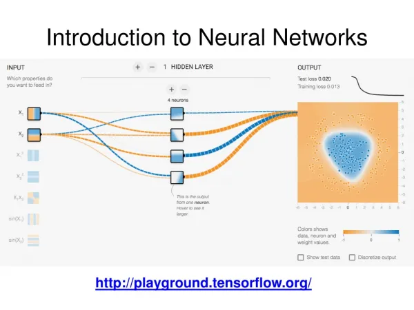
Artificial Intelligence Techniques. Introduction to Neural Networks 1. Aims: Section. fundamental theory and practical applications of artificial neural networks. Aims: Session Aim.

E N D
Artificial Intelligence Techniques Introduction to Neural Networks 1
Aims: Section fundamental theory and practical applications of artificial neural networks.
Aims: Session Aim Introduction to the biological background and implementation issues relevant to the development of practical systems.
Biological neuron • Taken from http://hepunx.rl.ac.uk/~candreop/minos/NeuralNets/neuralNetIntro.html
Human brain consists of approx.10 billion neurons interconnected with about 10 trillion synapses .
A neuron: specialized cell for receiving, processing and transmitting informations.
Electric charge from neighboring neurons reaches the neuron and they add.
The summed signal is passed to the soma thatprocessing this information.
The strength and polarity of the output depends features of each synapse
McCulloch-Pitts model X1 W1 Y X2 W2 T W3 X3 Y=1 if W1X1+W2X2+W3X3 T Y=0 if W1X1+W2X2+W3X3<T
McCulloch-Pitts model Y=1 if W1X1+W2X2+W3X3 T Y=0 if W1X1+W2X2+W3X3<T
Introduce the bias Take the threshold over to the other side of the equation and replace it with a weight W0 which equals -T, and include a constant input X0 which equals 1.
Introduce the bias Y=1 if W1X1+W2X2+W3X3 - T 0 Y=0 if W1X1+W2X2+W3X3 -T <0
Introduce the bias • Lets just use weights – replace T with a ‘fake’ input • ‘fake’ is always 1.
Introduce the bias Y=1 if W1X1+W2X2+W3X3 +W0X0 0 Y=0 if W1X1+W2X2+W3X3 +W0X0 <0
Logic functions - OR X0 -1 X1 Y 1 X2 1 Y = X1 OR X2
Logic functions - AND X0 -2 X1 Y 1 X2 1 Y = X1 AND X2
Logic functions - NOT X0 0 Y X1 -1 Y = NOT X1
The weighted sum • The weighted sum, Σ WiXi is called the “net” sum. • Net = Σ WiXi • y=1 if net 0 • y=0 if net < 0
Hard-limiter The threshold function is known as a hard-limiter. y 1 net 0 When net is zero or positive, the output is 1, when net is negative the output is 0.
Example Original image Weights -1 0 +1 +1 Net = 14
Example with bias With a bias of -14, the weighted sum, net, is 0. Any pattern other than the original will produce a sum that is less than 0. If the bias is changed to -13, then patterns with 1 bit different from the original will give a sum that is 0 or more, so an output of 1.
Generalisation • The neuron can respond to the original image and to small variations • The neuron is said to have generalised because it recognises patterns that it hasn’t seen before
Pattern space • To understand what a neuron is doing, the concept of pattern space has to be introduced • A pattern space is a way of visualizing the problem • It uses the input values as co-ordinates in a space
Pattern space in 2 dimensions X2 X1 X2 Y 0 0 0 0 1 0 1 0 0 1 1 1 1 The AND function 1 0 0 X1 1 0
Linear separability The AND function shown earlier had weights of -2, 1 and 1. Substituting into the equation for net gives: net = W0X0+W1X1+W2X2 = -2X0+X1+X2 Also, since the bias, X0, always equals 1, the equation becomes: net = -2+X1+X2
Linear separability The change in the output from 0 to 1 occurs when: net = -2+X1+X2 = 0 This is the equation for a straight line. X2 = -X1 + 2 Which has a slope of -1 and intercepts the X2 axis at 2. This line is known as a decision surface.
Linear separability X2 X1 X2 Y 0 0 0 0 1 0 1 0 0 1 1 1 2 1 The AND function 0 2 X1 1 0
Linear separability • When a neuron learns it is positioning a line so that all points on or above the line give an output of 1 and all points below the line give an output of 0 • When there are more than 2 inputs, the pattern space is multi-dimensional, and is divided by a multi-dimensional surface (or hyperplane) rather than a line
Are all problems linearly separable? • No • For example, the XOR function is non-linearly separable • Non-linearly separable functions cannot be implemented on a single neuron
Exclusive-OR (XOR) X2 X1 X2 Y 0 0 0 0 1 1 1 0 1 1 1 0 2 ? ? 1 0 2 X1 1 0
Learning • A single neuron learns by adjusting the weights • The process is known as the delta rule • Weights are adjusted in order to minimise the error between the actual output of the neuron and the desired output • Training is supervised, which means that the desired output is known
Delta rule The equation for the delta rule is: ΔWi = ηXiδ = ηXi(d-y) where d is the desired output and y is the actual output. The Greek “eta”, η, is a constant called the learning coefficient and is usually less than 1. ΔWi means the change to the weight, Wi.
Delta rule • The change to a weight is proportional to Xi and to d-y. • If the desired output is bigger than the actual output then d - y is positive • If the desired output is smaller than the actual output then d - y is negative • If the actual output equals the desired output the change is zero
Example • Assume that the weights are initially random • The desired function is the AND function • The inputs are shown one pattern at a time and the weights adjusted
Example Start with random weights of 0.5, -1, 1.5 When shown the input pattern 1 0 0 the weighted sum is: net = 0.5 x 1 + (-1) x 0 + 1.5 x 0 = 0.5 This goes through the hard-limiter to give an output of 1. The desired output is 0. So the changes to the weights are: W0 negative W1 zero W2 zero
Example New value of weights (with η equal to 0.1) of 0.4, -1, 1.5 When shown the input pattern 1 0 1 the weighted sum is: net = 1 x 0.4 + (-1) x 0 + 1.5 x 1 = 1.9 This goes through the hard-limiter to give an output of 1. The desired output is 0. So the changes to the weights are: W0 negative W1 zero W2 negative
Example New value of weights of 0.3, -1, 1.4 When shown the input pattern 1 1 0 the weighted sum is: net = 1 x 0.3 + (-1) x 1 + 1.4 x 0 = -0.7 This goes through the hard-limiter to give an output of 0. The desired output is 0. So the changes to the weights are: W0 zero W1 zero W2 zero
Example New value of weights of 0.3, -1, 1.4 When shown the input pattern 1 1 1 the weighted sum is: net = 1 x 0.3 + (-1) x 1 + 1.4 x 1 = 0.7 This goes through the hard-limiter to give an output of 1. The desired output is 1. So the changes to the weights are: W0 zero W1 zero W2 zero