Download
1 / 59
940 likes | 3.16k Views
CHEE 412 Partial Differential Equations in MATLAB. Hadis Karimi Queen’s University March 2011. Introduction. Parabolic partial differential equations are encountered in many chemical engineering applications MATLAB’s pdepe command can solve these

E N D
CHEE 412Partial Differential Equations in MATLAB Hadis Karimi Queen’s University March 2011
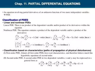
Introduction • Parabolic partial differential equations are encountered in many chemical engineering applications • MATLAB’s pdepe command can solve these • For partial dierential equations in two space dimensions PDE Toolbox can solve four types of equations: Elliptic, Parabolic, Hyperbolic and Eigenvalue
Agenda • Solving a parabolic PDE in MATLAB using “pdepe” function • A mass transfer example • A heat transfer example • Solving a system of parabolic PDE’s in MATLAB using “pdepe” function • A mass transfer example • Solving other types of PDE’s using PDE toolbox • A heat transfer example using PDE toolbox
PDE in One Space Dimension • The form of Parabolic PDE’s in MATLAB • Boundary conditions • Initial conditions m=0 for Cartesian, for cylindrical, 1 and for spherical 2
Initial Conditions X=L2 @ t=0
Boundary Conditions X=L3
Steps to Solve PDE’s in MATLAB 1- Define the system 2- Specify boundary conditions 3- Specify initial conditions 4- Write System m-file 5-Write Boundary Conditions m-file 6- Write Initial condition m-file 7-Write MATLAB script M-file that solves and plots
4- Write System m-file function [c,b,s] = system(x,t,u,DuDx) c = 1; b =D1*DuDx; s = 0; end
5-Write Boundary Conditions m-file function [pl,ql,pr,qr] = bc1(xl,ul,xr,ur,t) pl = 0; ql = 1/D1; pr = 0; qr = (D2-D1)/D1; end
6- Write Initial Conditions m-file function value = initial1(x) value = C0; end
7-Write MATLAB script M-file that solves and plots m = 0; %Define the solution mesh x = linspace(0,1,20); t = linspace(0,2,10); %Solve the PDE u = pdepe(m,@system,@initial1,@bc1,x,t); %Plot solution surf(x,t,u); title('Surface plot of solution.'); xlabel('Distance x'); ylabel('Time t');
Example 2: A Heat Transfer System L q” T=0 x
Defining System function [c,b,s]=pdecoef(x,t,u,DuDx) global rho cp k c=rho*cp; b=k*DuDx; s=0; end
Initial Conditions function u0=pdeic(x) u0=0; end
Boundary Conditions x=0 p=q” q=1 or Remember x=L p=T=ur q=0
Writing Boundary Condition m-file function[pl,ql,pr,qr]=pdebc(xl, ul,xr,ur,t) global q pl=q; ql=1; pr=ur; qr=0; end
Calling the Solver tend=10; m=0; x=linspace(0,L,200); t=linspace(0,tend,50); sol=pdepe(m,@pdecoef,@pdeic,@pdebc,x,t);
Plotting Temperature=sol(:,:,1); figure plot(t,Temperature(:,1))
Example 3: Mass Transport in the Saliva Layer Mucosa Blood Stream Saliva Drug Transport Direction Lozenge RL RS RM
Boundary Conditions Mucosa Blood Stream Saliva Drug Transport Direction Lozenge RL
Boundary Conditions Mucosa Blood Stream Saliva Drug Transport Direction Lozenge RS
Initial Conditions Mucosa Blood Stream Saliva Drug Transport Direction Lozenge Before any drug is released (at time = 0), the drug and glucose concentrations in the saliva are equal to zero: C1 =Cg =0
System function [c,b,s] = eqn (x,t,u,DuDx) c = [1; 1]; b = [D1; Dg] .* DuDx; s = [-kv*u(1); -kv*u(2)]; end
Boundary Conditions function [pl,ql,pr,qr] = bc2(xl,ul,xr,ur,t) pl = [D1*kd/D1g*(csolg-ul(2))*(rou1 -ul(1))); Dg*kd/Dgg*(csolg-ul(2))*(roug-ul(2)))]; ql = [-1; -1]; pr = [K1*ur(1)-c2Rs; Kg*ur(2)-cGRs]; qr = [0; 0]; end
Initial Conditions function value = initial2(x); value = [0;0]; end
Solving and Plotting m = 2; x = linspace(0,1,10); t = linspace(0,1,10); sol = pdepe(m,@eqn,@initial2,@bc2,x,t); u1 = sol(:,:,1); u2 = sol(:,:,2); subplot(2,1,1) surf(x,t,u1); title('u1(x,t)'); xlabel('Distance x'); ylabel('Time t'); subplot(2,1,2) surf(x,t,u2); title('u2(x,t)'); xlabel('Distance x'); ylabel('Time t');
Single PDE in Two Space Dimensions 1. Elliptic 2. Parabolic 3. Hyperbolic 4. Eigenvalue
Example 4 No Heat T=0 T=10 Laplace’s Equation No Heat
Step 1 • Start the toolbox by typing in >> pdetool at the Matlab prompt
Step 8 Specify Boundary Condition Steps 9 - 10 Select Boundary 1 and specify condition