Download
1 / 62
760 likes | 1.19k Views
Image Restoration. CONTENT. Introduction and Overview n(r,c) – additive noise function Noise Models Gaussian Salt-and-pepper Uniform Rayleigh Noise Removal using Spatial Filters Order filters Mean filters h(r,c) - degradation Function Geometric Transforms. Introduction .

E N D
CONTENT • Introduction and Overview • n(r,c) – additive noise function • Noise Models • Gaussian • Salt-and-pepper • Uniform • Rayleigh • Noise Removal using Spatial Filters • Order filters • Mean filters • h(r,c) - degradation Function • Geometric Transforms
Introduction • IR – process of finding an approximation to the degradation process and finding the appropriate inverse process to estimate the original image • IR differ IE – it used a mathematical model for image degradation
Overview • Types of degradation :- • Blurring caused by motion or atmospheric disturbance • Geometric distortion caused by imperfect lenses • Superimposed interference patterns caused by mechanical systems • Spatial quantization • Noise from electronic sources h(r,c) = degradation function n(r,c) = additive noise function
IR process (fig 9.1-1) • We see that sample degraded images and knowledge of the image acquisition process are inputs to development of a degradation model • After the model has been developed, the next step is the formulation of the inverse process • This inverse degradation process is then applied to the degraded image, d(r,c), which results in the output image, Î(r,c), • The output image Î(r,c), is the restored image which represents an estimate of original image, I(r,c)
Once the estimated image has been created, any knowledge gained by observation & analysis of this image is used as additional input for further development of degradation model • This process continues until satisfactory results are achieved
System Model • Degradation process model consists of 2 parts, the degradation function & the noise function • General mode in spatial domain : d(r,c) = h(r,c) * I(r,c) + n(r,c) where d(r,c) = degraded image h(r,c) = degradation function I(r,c) = original image n(r,c) = additive noise function
System Model (cont’d) • Frequency domain : D(u,v) = H(u,v) * I(u,v) + N(u,v) where D(u,v) = Fourier transform of the degraded image H(u,v) = Fourier transform of the degradation function I(u,v) = Fourier transform of the original image N(u,v) = Fourier transform of the additive noise function
Noise Models • Any undesired information that contaminates an image • noise models is a random variable with a probability density function (PDF) that describes its shape and distribution • The actual distribution of noise in a specific image is the histogram of the noise • Noise can be modeled with Gaussian (“normal”), uniform, salt-and-pepper (“impulse”), or Rayleigh distribution
Gaussian model – occur from electronic noise in image acquisition system • Most problematic with poor lighting conditions or vary high temperatures • Also valid for film grain noise • Salt-and-pepper noise (also called impulse noise, shot noise or spike noise) typically caused by malfunctioning pixel element in camera sensors, faulty memory locations, or timing errors in digitization process
Uniform noise is useful - it can be used to generate any other type of noise distribution, and is often used to degrade images for the evaluation of image restoration algo since provides the most unbiased or neutral noise model
A bell-shapped • 70% of all values fall within the range from one standard deviation (σ) below the mean (m) to one above • About 95% fall within two standard deviations
Uniform distribution • The gray level values of the noise are evenly distributed across a specific range
Salt-and-pepper • There are only 2 possible values, a and b, and the probability of each is typically less than 0.2 – with numbers greater than this the noise will swamp out the image
image with added Gaussian noise with mean = 0 and variance = 600, and its histogram
image with added uniform noise with mean = 0 and variance = 600, and its histogram
image with added salt-and-pepper noise with the probability of each 0.08, and its histogram
Noise Removal Using Spatial Filters • Spatial filters can be effectively used to remove various types of noise • Operate on small neighborhoods, 3x3 to 11x11 • Will use the degradation model with the assumption that h(r,c) causes no degradation where the only corruption to the image is caused by additive noise
d(r,c) = I(r,c) + n(r,c) where d(r,c) = degraded image I(r,c) = original image n(r,c) = additive noise function
Two primary categories; order filters and mean filters • Order filters – implemented by arranging the neighborhood pixels in order from smallest to largest gray level value, and using this ordering to select the “correct” value • Mean filters determine, in one sense or another, an average value
Mean filters work best with Gaussian or uniform noise • Order filters work best with salt-and-pepper, negative exponential, or Rayleigh noise • Mean filters have disad of blurring the image edges, or details • Order filters such as mean can be used to smooth images
Order Filters • Operate on small subimages, windows, and replace the center pixel value (similar to convolution process) • Given an N x N wondow, W, the pixel values can be ordered as follows
(85, 88, 95, 100, 104, 104, 110, 110, 114) • Min = 85, Med = 104, max = 114 (will be replaced at the center value) • Median filter is most useful • Max & min filters can eliminate salt or pepper noise
a) Image with added salt-and-pepper noise, the probability for salt = probability for pepper = 0.10, b) after median filtering with a 3x3 window, all the noise is not removed a) b)
c) after median filtering with a 5x5 window, all the noise is removed, but the image is blurry acquiring the “painted” effect c)
Two order filters are midpoint and alpha-trimmed mean filters – both order and mean filters since they rely on ordering the pixels values, but are then calculated by an averaging process • Midpoint filter – the average of max & min within the window; • Most useful for Gaussian & uniform noise
Alpha-trimmed mean is the average of pixel values within the window, but with some of the endpoint ranked excluded • Useful for images containing multiple types of noise, Gaussian and salt-and-pepper noise where T is the number of pixel values excluded at each end of the ordered set, and can range from 0 to (N2 – 1)/2
Alpha-trimmed mean filter ranges from a mean to median filter, depending on the value selected for the T parameter
Exercise Apply the following filters to the 3 x 3 subimages below, and find the output for each: (a) median, (b) maximum, (c) minimum, (d) midpoint, (e) alpha-trimmed mean with T = 2.
Figure 9.3-5 Alpha-Trimmed Mean. This filter can vary between a mean filter and a median filter. a) Image with added noise: zero-mean Gaussian noise with a variance of 200, and salt-and-pepper noise with probability of each = 0.03, b) result of alpha-trimmed mean filter, mask size = 3x3, T = 1, c) result of alpha-trimmed mean filter, mask size = 3x3, T = 2, d) result of alpha-trimmed mean filter, mask size = 3x3, T = 4. As the T parameter increases the filter becomes more like a median filter, so becomes more effective at removing the salt-and pepper noise. a) b) c) d)
Mean Filters • Function by finding some form of an average within the NxN window, using sliding window concept to process entire image • The most basic – arithmetic mean filter which finds the arithmetic average of pixel values ; where N2 = the number of pixels in the NxN window, W • Smooths out local variations & work best with Gaussian, gamma and uniform noise
Contra-harmonic mean filter works well for images containing salt OR pepper type noise, depending on the filter order, R: where W is the NxN window under consideration • Negative values of R, eliminates salt-type noise • Positive values, eliminates pepper-type noise
Geometric mean filter works best with Gaussian noise, & retains detail information better than an arithmetic mean filter • Defined as the product of pixel values within window, raised to the 1/N2 power:
Harmonic mean filter also fails with pepper noise but works well for salt noise; • Retaining detail information better than the arithmetic mean filter
Exercise Apply the following filters to the 3 x 3 subimages below, and find the output for each: (a) arithmetic mean, (b) contra-harmonic mean with R= -2, (c) contra-harmonic mean with R=+2, (d) geometric mean, (e) harmonic mean, (f) Yp mean with P = -1, (g) Yp mean with P = +2.
The Degradation Function • Either spatially-invariant or spatially-variant • Spatially-invariant degradation affects all pixels in the image same • Eg, poor lens focus and camera motion • Spatially-variant degradation depend on spatial location & more difficult to model • Eg, imperfects in a lens or object motion
Point Spread Function • d(r,c) = I(r,c) * h(r,c) where * denotes the convolution process • h(r,c) is called point spread function (PSF), or blur function • PSF of a linear, spatially-invariant(shift invariant) system can be empirically determined by imaging a single point of light
Estimation of the Degradation Function • Estimated primarily by combinations of • Image analysis • Experimentation • Mathematical modeling • Image analysis : examine a known point or line in an image, and estimate the PSF by measuring the width and distribution of known feature in blurred image
Experimentation : • PSF can be found by imaging a point of light • A more reliable method is to use sinusoidal inputs at many different spatial frequencies to find the H(u,v) • Mathematical modeling examples: • The motion blur model • Atmospheric turbulence degradation model used in astronomy and remote sensing
Geometric Transforms • Spatially-variant • Images that have been spatially, or geometrically, distorted • Used to modify the location of pixel values within an image, typically to correct images that have been spatially warped • Often referred as rubber-sheet transforms - image is modeled as a sheet of rubber and stretched and shrunk