Download
1 / 18
220 likes | 503 Views
Image Restoration. Comp344 Tutorial Kai Zhang. Outline. DIPUM Tool box Noise models Periodical noise and removal Noise parameter estimation Spatiral noise removal. The DIPUM Tool box. M-functions from the book Digital Image Processing Using MATLAB

E N D
Image Restoration Comp344 Tutorial Kai Zhang
Outline • DIPUM Tool box • Noise models • Periodical noise and removal • Noise parameter estimation • Spatiral noise removal
The DIPUM Tool box • M-functions from the book Digital Image Processing Using MATLAB • http://www.imageprocessingplace.com/DIPUM_Toolbox_1/dipum_toolbox_main_page.htm • Freedownload • No original m-functions • But can still used for demo
Noise models • Given a random number generator, how to generate random numbers with a pre-specified CDF? • Suppose the random number w is in [0,1] • We want to generate a Rayleigh distributed sample set • To find z solve the following equation
Functions • Function r = imnoise(f, type, parameters) • Corrupt image f with noise specified in type and parameters • Results returned in r • Type include: uniform, gaussian, salt & pepper, lognormal, rayleigh, exponential • Function r = imnoise2(type, M,N,a,b); • Generates arrar r of size M-by-N, • Entries are of the specified distribution type • A and b are parameters
Codes • Code1 • f = imread('lenna.jpg'); • g = imnoise(f, 'gaussian', 0, 0.01); • figure, imshow(g); • g = imnoise(f, 'salt & pepper', 0.01); • figure, imshow(g); • Code2 • r = imnoise2('gaussian',10000,1,0,1); • p = hist(r,50); • bar(p);
Periodical spatial noise • Model • Using 2-d sinusoid functions • M, N: image size • A: magnitude of noise • U0, v0: frequency along the two directions • Bx, By: phase displacement • Observation: when x goes through 0,1,2,…,M, the left term will repeat u0 times. So the horizontal frequency is u0. Similar for v0.
Function: [r, R, S] = imnoise3(M,N, C, A, B); • Generate a sinusoide noise pattern r • Of size M by N • With Fourier transform R • And spectrum S • C is a K-by-2 matrix, each row being coordinate (u,v) of an impulse • A 1-by-K contains the amplitude of each impulse • B is K-by-2 matrix each row being the phase replacement
Codes • C = [0 64; 0 128; 32 32; 64 0; 128 0; -32 32]; • [r, R, S] = imnoise3(256,256,C); • figure,imshow(S,[]); • figure,imshow(r,[]);
Noise estimation • How to determine type and parameters of noise given an image f corrupted by noise? • Step 1. Manually choosing a region as featureless as possible, so that variability is primarily due to noise. [B,c,r] = roipoly(f); • Step2. compute the histogram of the selected image patch [p, npix] = histroi(f, c, r); • Step3. determine the noise type through observation • Step4. estimating the central moments [v, unv] = statmoments(p, 2);
Functions • Function: [B,c,r] = roipoly(f); • F is the image • C and r are sequential column and row coordinates of the polygon / can also be specified by the mouse • B is the region selected (of value 1), and all the rest part of the image is 0 • Function [p, npix] = histroi(f, c,r); • Generating histogram p of the region of interest(ROI) specified in c and r (vertex coordinates)
codes • f = imread(‘lenna.jpg’); • noisy_f = imnoise(f,'gaussian',0,0.01); • figure,imshow(noisy_f,[]); • [B, c, r] = roipoly(noisy_f); %needs mouse interations • figure,plot(B); • [p,npix] = histroi(f,c,r); • figure,bar(p,1); • [v, unv] = statmoments(p,2); • X = imnoise2('gaussian', npix,1,unv(1),unv(2)^0.5); figure, hist(X,100);
Spatial noise removal • Function f = spfilter(g, type, m, n, parameter); • Performs spatial filtering • Type include: amean, gmean, hmean, chmean, median, max, min, midpoint, artimmed
Codes • Creating a salt noise image • f = imread('lenna.jpg'); • R = imnoise2('salt & pepper', M, N, 0.1, 0); • c = find(R == 0); • gp = f; • gp(c) = 0; • figure, imshow(gp); • Filtering • fp = spfilt(gp, 'chmean', 3, 3, 1.5); • fpmax = spfilt(gp, 'max',3,3); • figure,imshow(fp); • figure,imshow(fpmax);