Download

1 / 58
670 likes | 722 Views
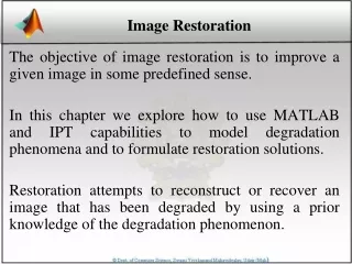
Image Restoration. Preview. Goal of image restoration Improve an image in some predefined sense Difference with image enhancement ? Features Image restoration v.s image enhancement Objective process v.s. subjective process A prior knowledge v.s heuristic process

E N D
Preview • Goal of image restoration • Improve an image in some predefined sense • Difference with image enhancement ? • Features • Image restoration v.s image enhancement • Objective process v.s. subjective process • A prior knowledge v.s heuristic process • A prior knowledge of the degradation phenomenon is considered • Modeling the degradation and apply the inverse process to recover the original image
Preview (cont.) • Target • Degraded digital image • Sensor, digitizer, display degradations are less considered • Spatial domain approach • Frequency domain approach
Outline • A model of the image degradation / restoration process • Noise models • Restoration in the presence of noise only– spatial filtering • Periodic noise reduction by frequency domain filtering • Linear, position-invariant degradations • Estimating the degradation function • Inverse filtering
A model of the image degradation/restoration process g(x,y)=f(x,y)*h(x,y)+h(x,y) G(u,v)=F(u,v)H(u,v)+N(u,v)
Noise models 雜訊模型 • Source of noise • Image acquisition (digitization) • Image transmission • Spatial properties of noise • Statistical behavior of the gray-level values of pixels • Noise parameters, correlation with the image • Frequency properties of noise • Fourier spectrum • Ex. white noise (a constant Fourier spectrum)
Noise probability density functions • Noises are taken as random variables • Random variables • Probability density function (PDF)
Gaussian noise • Math. tractability in spatial and frequency domain • Electronic circuit noise and sensor noise mean variance Note:
Gaussian noise (PDF) 70% in [(m-s), (m+s)] 95% in [(m-2s), (m+2s)]
Uniform noise • Less practical, used for random number generator Mean: Variance:
Impulse (salt-and-pepper) nosie • Quick transients, such as faulty switching during imaging If either Pa or Pb is zero, it is called unipolar. Otherwise, it is called bipoloar. • In practical, impulses are usually stronger than image • signals. Ex., a=0(black) and b=255(white) in 8-bit image.
Test for noise behavior • Test pattern Its histogram: 0 255
Periodic noise • Arise from electrical or electromechanical interference during image acquisition • Spatial dependence • Observed in the frequency domain
Sinusoidal noise: Complex conjugate pair in frequency domain
Estimation of noise parameters • Periodic noise • Observe the frequency spectrum • Random noise with unknown PDFs • Case 1: imaging system is available • Capture images of “flat” environment • Case 2: noisy images available • Take a strip from constant area • Draw the histogram and observe it • Measure the mean and variance
Observe the histogram uniform Gaussian
Measure the mean and variance • Histogram is an estimate of PDF Gaussian: m, s Uniform: a, b
Outline • A model of the image degradation / restoration process • Noise models • Restoration in the presence of noise only – spatial filtering • Periodic noise reduction by frequency domain filtering • Linear, position-invariant degradations • Estimating the degradation function • Inverse filtering
Additive noise only g(x,y)=f(x,y)+h(x,y) G(u,v)=F(u,v)+N(u,v)
Spatial filters for de-noising additive noise • Skills similar to image enhancement • Mean filters • Order-statistics filters • Adaptive filters
Mean filters • Arithmetic mean • Geometric mean Window centered at (x,y)
Noisy Gaussian original m=0 s=20 Arith. mean Geometric mean
Mean filters (cont.) • Harmonic mean filter • Contra-harmonic mean filter Q=-1, harmonic Q=0, airth. mean Q=+, ?
Pepper Noise 黑點 Salt Noise 白點 Contra- harmonic Q=-1.5 Contra- harmonic Q=1.5
Wrong sign in contra-harmonic filtering Q=1.5 Q=-1.5
Order-statistics filters • Based on the ordering(ranking) of pixels • Suitable for unipolar or bipolar noise (salt and pepper noise) • Median filters • Max/min filters • Midpoint filters • Alpha-trimmed mean filters
Order-statistics filters • Median filter • Max/min filters
bipolar Noise Pa = 0.1 Pb = 0.1 3x3 Median Filter Pass 1 3x3 Median Filter Pass 2 3x3 Median Filter Pass 3
Salt noise Pepper noise Min filter Max filter
Order-statistics filters (cont.) • Midpoint filter • Alpha-trimmed mean filter • Delete the d/2 lowest and d/2 highest gray-level pixels Middle (mn-d) pixels
Uniform noise Left + Bipolar Noise Pa = 0.1 Pb = 0.1 m=0 s2=800 5x5 Arith. Mean filter 5x5 Geometric mean 5x5 Median filter 5x5 Alpha-trim. Filter d=5
Adaptive filters • Adapted to the behavior based on the statistical characteristics of the image inside the filter region Sxy • Improved performance v.s increased complexity • Example: Adaptive local noise reduction filter
Adaptive local noise reduction filter • Simplest statistical measurement • Mean and variance • Known parameters on local region Sxy • g(x,y): noisy image pixel value • s2h: noise variance (assume known a prior) • mL : local mean • s2L: local variance
Adaptive local noise reduction filter (cont.) • Analysis: we want to do • If s2h is zero, return g(x,y) • If s2L> s2h , return value close to g(x,y) • If s2L= s2h , return the arithmetic mean mL • Formula
Gaussian noise Arith. mean 7x7 m=0 s2=1000 Geometric mean 7x7 adaptive
Outline • A model of the image degradation / restoration process • Noise models • Restoration in the presence of noise only – spatial filtering • Periodic noise reduction by frequency domain filtering • Linear, position-invariant degradations • Estimating the degradation function • Inverse filtering
Periodic noise reduction • Pure sine wave • Appear as a pair of impulse (conjugate) in the frequency domain
Periodic noise reduction (cont.) • Bandreject filters • Bandpass filters • Notch filters • Optimum notch filtering
Bandreject filters * Reject an isotropic frequency ideal Butterworth Gaussian
noisy spectrum filtered bandreject
Bandpass filters • Hbp(u,v)=1- Hbr(u,v)
Notch filters • Reject(or pass) frequencies in predefined neighborhoods about a center frequency ideal Butterworth Gaussian
Horizontal Scan lines Notch pass DFT Notch pass Notch reject
Outline • A model of the image degradation / restoration process • Noise models • Restoration in the presence of noise only – spatial filtering • Periodic noise reduction by frequency domain filtering • Linear, position-invariant degradations • Estimating the degradation function • Inverse filtering
A model of the image degradation /restoration process g(x,y)=f(x,y)*h(x,y)+h(x,y) G(u,v)=F(u,v)H(u,v)+N(u,v) If linear, position-invariant system
Linear, position-invariant degradation Properties of the degradation function H • Linear system • H[af1(x,y)+bf2(x,y)]=aH[f1(x,y)]+bH[f2(x,y)] • Position(space)-invariant system • H[f(x,y)]=g(x,y) • H[f(x-a, y-b)]=g(x-a, y-b) • c.f. 1-D signal • LTI (linear time-invariant system)
Linear, position-invariant degradation model • Linear system theory is ready • Non-linear, position-dependent system • May be general and more accurate • Difficult to solve compuatationally • Image restoration: find H(u,v) and apply inverse process • Image deconvolution