Download
1 / 30
330 likes | 356 Views
Image Restoration. The objective of image restoration is to improve a given image in some predefined sense. In this chapter we explore how to use MATLAB and IPT capabilities to model degradation phenomena and to formulate restoration solutions.

E N D
Image Restoration The objective of image restoration is to improve a given image in some predefined sense. In this chapter we explore how to use MATLAB and IPT capabilities to model degradation phenomena and to formulate restoration solutions. Restoration attempts to reconstruct or recover an image that has been degraded by using a prior knowledge of the degradation phenomenon.
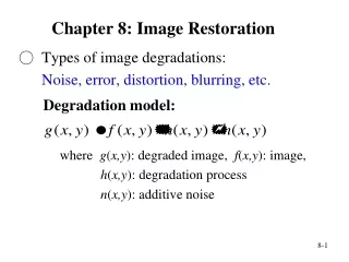
Image Restoration A model of image Degradation/Restoration process: The degradation process is modeled as a degradation function that, together with an additive noise term, operates on an input image f(x, y) to produce a degraded image. g(x, y) = H [ f (x, y)] + η(x, y) Given g(x, y), some knowledge about the degradation function H, and some knowledge about the additive term noise η(x, y). The objective of the restoration is to obtain an estimate, f(x, y), of the original image.
Image Restoration A model of image Degradation/Restoration process:
Image Restoration A model of image Degradation/Restoration process: In spatial domain processing, it can be shown that the degraded image g(x, y) = h(x, y) * f (x, y) + η(x, y) In equivalent frequency domain representation: G(u, v) = H(u, v) F(u, v) + N(u, v)
Image Restoration A model of image Degradation/Restoration process: Example: >>f=imread(‘moon.tif’); >>len=31; >>theta=11; >>psf=fspecial(‘motion’,len,theta); >>blur=imfilter(f,psf,’circular’,’conv’); >>imshow(blur) >>wnr1=deconvwnr(blur,psf); >> figure, imshow(wnr1);
Image Restoration Noise models: The ability to simulate the behavior and effects of noise is central to image restoration. In this chapter we will see two basic steps of noise models 1) noise in the spatial domain 2) noise in the frequency domain
Image Restoration Function imnoise: The toolbox uses the function imnoise to corrupt an image with noise. This function has the following syntax: g = imnoise(f, type, parameters) where f is the input image, and type are as follows: 1) gaussian 2) localvar 3) salt & papper 4) speckle 5) poisson
Image Restoration Function imnoise: g = imnoise(f, ‘gaussian’, m, var) adds Gaussian noise of mean m and variance var to image f. The default is zero mean noise with 0.01 variance. g = imnoise(f, ‘localvar’, v) Adds zero mean, Gaussian noise of local variance, v, to image f. g = imnoise(f, 'poisson') generates Poisson noise from the data instead of adding artificial noise to the data.
Image Restoration Function imnoise: g = imnoise(f,'salt & pepper',d) adds salt and pepper noise to the image f, where d is the noise density. g = imnoise(f, ‘speckle',v) adds multiplicative noise to the image f, using the equation g = f+n*f, where n is uniformly distributed random noise with mean 0 and variance v. The default for v is 0.04.
Image Restoration Function imnoise: >>imread(‘eight.tif’); >>g=imnoise(f,’gaussian’); >>v=double(g); >>g1=imnoise(f,’localvar’,v); >>g2=imnoise(f,’poisson’); >>g3=imnoise(f, ‘salt & pepper); >>g4=imnoise(f, ‘speckle); display g, g1, g2, g3 and g4.
Image Restoration Function imnoise: >>I = imread('eight.tif'); >>imshow(I) >>J = imnoise(I,'salt & pepper',0.02); >>figure, imshow(J) >>K = filter2(fspecial('average',3),J)/255; >>figure, imshow(K) >>L = medfilt2(J,[3 3]); >>figure, imshow(L)
Geometric Transformation & Image Registration Geometric transformation modifies the spatial relationship between the pixels in an image. They are often called rubber-sheet transformations because they may be viewed as printing an image on a sheet of rubber and then stretching this sheet according to a predefined set of rules. Geometric transformations are frequently used to perform image registration, a process that takes two images of the same scene and aligns them so they can be merged for visualization, or for quantitative comparison.
Geometric Transformation & Image Registration Geometric Spatial Transformation: Consider an image f, defined over a (w, z) coordinate system, undergoes geometric distortion to produce an image g, defined over an (x, y) coordinate system. This transformation may be expressed as (x, y) = T { (w, z) } for example, if (x, y) = T{(w, z)} = (w/2, z/2), the distortion is simply a shrinking of f by half in the both spatial dimensions T{(5,2)} = (2.5, 1)
Geometric Transformation & Image Registration One of the most commonly used spatial transformations is affine transformation.
Geometric Transformation & Image Registration For example, one way to create an affine tform is to provide T matrix directly, >>T=[2 0 0; 0 3 0; 0 0 1]; >>tform = maketform(‘affine’, T); >> tform ndim_in = 2 ndim_out=2 forward_fcn=@fwd_affine inverse_fcn=@inv_affine tdata = [1x1 struct]
Geometric Transformation & Image Registration Applying Spatial Transformations to images: Most computational methods for spatially transforming an image fall into one of two categories: 1) forward mapping 2) Inverse mapping Methods based on forward mapping scan each input pixel in turn, copying its value into the output image at the location determined by T{(w,z)}. 2) An inverse mapping Methods based on scan each input pixel in turn, copying its value into the output image at the location determined by T-1{(w,z)}.
Geometric Transformation & Image Registration >>f=checkerboard(50); >> s=0.8; >> theta=pi/6; >> T=[s*cos(theta) s*sin(theta) 0; -s*sin(theta) s*cos(theta) 0; 0 0 1]; >> tform=maketform('affine', T); >> g=imtransform(f,tform); >> imshow(f) >> figure, imshow(g)
Geometric Transformation & Image Registration Make and apply an affine transformation. T = maketform('affine',[.5 0 0; .5 2 0; 0 0 1]); tformfwd([10 20],T) I = imread('cameraman.tif'); I2 = imtransform(I,T); imshow(I2)
Geometric Transformation & Image Registration This example reads eight.tif, and rotates the the image to bring it into horizontal alignment. A rotation of 11 degree is all that is required. I = imread(‘eight.tif'); I = mat2gray(I); J = imrotate(I,11,'bilinear','crop'); imshow(I) figure, imshow(J)
Geometric Transformation & Image Registration This example reads eight.tif, and rotates the the image to bring it into resize to its 2 times larger is all that is required. I = imread(‘eight.tif'); I = mat2gray(I); J = imresize(I,2); imshow(I) figure, imshow(J)
Image Registration Image registration is the process of aligning two or more images of the same scene. Typically, one image, called the base image, is considered the reference to which the other images, called input images, are compared. The object of image registration is to bring the input image into alignment with the base image by applying a spatial transformation to the input image.
Image Registration Image registration is often used as a preliminary step in other image processing applications. For example, you can use image registration to align satellite images of the earth's surface or images created by different medical diagnostic modalities (MRI and SPECT). After registration, you can compare features in the images to see how a river has migrated, how an area is flooded, or to see if a tumor is visible in an MRI or SPECT image.
Image Registration I = checkerboard; J = imrotate(I,30); base_points = [11 11; 41 71]; input_points = [14 44; 70 81]; cpselect(J,I,input_points,base_points)
Registration in the presence of noise only When the only degradation present in noise, then it follows from the model g(x,y)=f(x,y)+n(x,y) Spatial Noise Filter: The spfilt performs filtering in the spatial domain with any filters types. And the function imlincomb use to compute the linear combination of the inputs, and has the following syntax B=imlincomb(c1,A1,c2,A2….) where c’s are real, double scalars, and A’s are numeric arrays of the same class and size.
Registration in the presence of noise only f=imread(‘eight.tif’) [M, N]=size(f); R=imnoise2(‘salt & pepper’,M,N,0.1,0); c=find(R==0); gp=f; gp(c)=0; imshow(R); figure, imshow(gp); R=imnoise2(‘salt & pepper’,M,N,0,0.1); c=find(R==1);
Registration in the presence of noise only gs=f; gs(c)=255; figure, imshow(gs); fp=spfilt(gp,’chmean’,3,3,1.5); fs=spfilt(gs,’chmean’,3,3,-1.5); display fp and fs.
Registration in the presence of noise only Adaptive Spatial Filters: The filters adopted without regard for how image characteristic vary from one location to another. The adaptive filters can be implement in MATLAB and the algorithm: Zmin=Minimum intensity value of Sxy Zmax=Maximum intensity value of Sxy Zmed=Median of intensity value of Sxy Zxy= Intensity value at coordinate (x,y) The adpmedian is use to implement this algorithm.
Registration in the presence of noise only Adaptive Spatial Filters: f=imread(‘eight.tif’); g=imnoise(f,’salt & pepper’,0.25); f1=medfilt2(g,[7 7],’symmetric’); f2=adpmedian(g,7); imshow(f1); figure, imshow(f2);
Periodic Noise Reduction by Frequency Domain Processing The periodic noise manifests itself as impulse-like that often are visible in the Fourier spectrum. The main approach for filtering these components is via notch filtering, the transfer function notch filter of order n is given by
Periodic Noise Reduction by Frequency Domain Processing Design and plot an IIR notch filter with 11 notches (equal to filter order plus 1) that removes a 60 Hz tone (f0) from a signal at 600 Hz (fs). For this example, set the Q factor for the filter to 35 and use it to specify the filter bandwidth. >>fs = 600; fo = 60; q = 35; bw = (fo/(fs/2))/q; >>[b,a] = iircomb(fs/fo,bw,'notch'); >>fvtool(b,a);