Download
1 / 110
1.1k likes | 1.13k Views
Learn how to improve degraded images using MATLAB and IPT models. Understand the image degradation process and formulate restoration solutions. Explore noise models and simulate their effects using MATLAB's imnoise function.

E N D
Chapter 5 Image Restoration Objectives: To improve a given image in some predefined sense How MATLAB and IPT models degradation phenomena and formulate restoration solutions. Image restoration is an objective process while image enhancement is subjective.
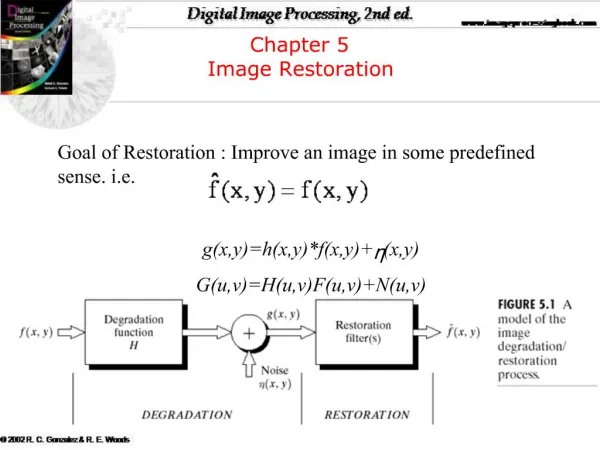
A Model of the Image Degradation/Restoration Process The degradation process is modeled as a degradation function that together with an additive noise term, operates on an input image f(x,y) to produce a degraded image g(x,y): Given g(x,y), some knowledge about the degradation function H, and some knowledge about the additive noise term , the objective of restoration is to obtain an estimate, , of the original image as close as possible to the original input image.
A Model of the Image Degradation/Restoration Process If H is a linear, spatially invariant process, it can be shown that the degraded image is given in the spatial domain by: Where h(x,y) is the spatial representation of the degradation function and “*” indicates convolution. We can also write its frequency domain equivalent as: Where all terms in capital letter refer to Fourier transform of corresponding terms. The degradation function H(u,v) is called the optical transform function (OTF), and the h(x,y) is called the point spread function. MATLAB provides conversion functions: otf2psfand psf2otf.
A Model of the Image Degradation/Restoration Process Because the degradation due to a linear, spatially invariant degradation function, H, can be modeled as convolution, sometimes the degradation process is referred to as “convolving the image with a PSF or OTF”. Similarly the restorationprocess is sometimes referred to as deconvolution. We first deal with cases where H is assumed to be an identity operator, so it does not have any effect on the process. This way we deal only with degradation noise. Later we get H involve too.
Noise Models • Ability to simulate the behavior and effects of noise is crucial to image restoration. • We will look at two noise models: • Noise in the spatial domain (described by the noise probability density function), and • Noise in the frequency domain, described by various Fourier properties of the noise. • MATLAB uses the function imnoise to corrupt an image with noise. This function has the basic syntax: • g = imnoise(f, type, parameters) • Where f is the input image, and type and parameters will be described later.
Adding Noise with Function imnoise Function imnoiseconverts the input image to class double in the range [0, 1] before adding noise to it. This is very important to remember. For example, to add Gaussian noise of mean 64 and variance 400 to a uint8 image, we scale the mean to 64/255 and the variance to 400/2552 for input into imnoise. Below is a summary of the syntax for this function (see Page 143 for more information) g = imnoise(f, ‘gaussian’, m, var) g = imnoise(f, ‘localvar’, V) g = imnoise(f, ‘localvar’, image_intensity, var) g = imnoise(f, ‘salt & pepper’, d) g = imnoise(f, ‘speckle’, var) g = imnoise(f, ‘poisson’)
Example: On the left the original image. On the right: g = imnoise(f, 'gaussian', 127/255, 0); Note that I have set the variance to 0, that is practically un- realistic. But for the sake of this example, we will let that go.
Example: On the left: g = imnoise(f, 'gaussian', 54/255, 200); On the right: g = imnoise(f, 'gaussian', 0, 200);
Generating Spatial Random Noise with a Specified Distribution Often, we wish to generate noise of types and parameters other than the ones listed on previous page. In such cases, spatial noise are generated using random numbers, characterized by probability density function (PDF) or by the corresponding cumulative distribution function (CDF). Two of the functions used in MATLAB to generate random numbers are: rand – to generate uniform random numbers, and randn – to generate normal (Gaussian) random numbers.
Example: Assume that we have a random number generator that generates numbers, w, uniformly in the [0 1] range. Suppose we wish to generate random numbers with a Rayleigh CDF, which is defined as: To find z we solve the equation: Or Since the square root term is nonnegative, we are assured that no values of z less than a are generated. In MATALB: R = a + sqrt(b*log(1 – rand(M, N) ));
Function imnoise2 generates random numbers having CDFs shown in the table below. They all use rand as: rand(M,N)
imnoise vs. imnoise2 The imnoise function generates a 1D noise array, imnoise2 will generate an M-by-N noise array. imnoise scales the noise array to [0 1], imnoise2 does not scale at all and will produce the noise pattern itself. The user specifies the parameters directly. Note: The salt-and-pepper noise has three values: 0 corresponding to pepper noise 1 corresponding to salt noise, and 0.5 corresponding to no noise. You can copy the imnoise2 function from the course web page.
r = imnoise2('gaussian', 100000, 1, 0, 1); p = hist(r, 50); bar(p)
r = imnoise2('gaussian', 256, 256, 0, 255); p = hist(r, 50); bar(p)
r = imnoise2(‘uniform', 100000, 1, 0, 1); p = hist(r, 50); bar(p)
r = imnoise2(‘lognormal', 100000, 1, 1, 0.25); p = hist(r, 50); bar(p)
r = imnoise2(‘rayleigh', 100000, 1, 1, 0.25); p = hist(r, 50); bar(p)
r = imnoise2(‘exponential', 100000, 1, 1, 1); p = hist(r, 50); bar(p) Does not matter
r = imnoise2(‘erlang', 100000, 1, 2, 5); p = hist(r, 50); bar(p)
r = imnoise2(‘salt & pepper', 100000, 1, 0.05, 0.05); p = hist(r, 50); bar(p) If r(x,y) = 0, black If r(x,y) = 1, white If r(x,y) = 0.5 none
Periodic Noise This kind of noise usually arises from electrical and/or electromagnetical interference during image acquisition. These kinds of noise are spatially dependent noise. The periodic noise is handled in an image by filtering in the frequency domain. Our model for a periodic noise is: Where A is amplitude, u0and v0determine the sinusoidal frequencies with respect to the x- and y-axis, respectively, and Bx and By are phase displacements with respect to the origin. The M-by-N DFT of the equation is:
This statement shows a pair of complex conjugate impulses located at (u+u0 , v+v0) and (u-u0 , v-v0), respectively. A MATLAB function (imnoise3) accepts an arbitrary number of impulse locations (frequency coordinates), each with its own amplitude, frequencies, and phase displacement parameters, and computes r(x, y) as the sum of sinusoids of the form shown in the previous page. The function also outputs the Fourier transform of the sum of sinusoides, R(u,v) and the spectrum of R(u,v). The sine waves are generated from the given impulse location information via the inverse DFT. Only one pair of coordinates is required to define the location of an impulse. The program generates the conjugate symmetric impulses.
C = [0 64; 0 128; 32 32; 64 0; 128 0; -32 32]; [r, R, S] = imnoise3(512, 512, C); imshow(S, []); C is k-by-2 matrix containing K pairs of frequency domain coordinates (u,v) r is the noise pattern of size M-by-N R is the Fourier transform of r S is the spectrum of R
u v [-32,0] [0,0] [32,0]
C = [0 32; 0 64; 16 16; 32 0; 64 0; -16 16]; [r, R, S] = imnoise3(512, 512, C); imshow(S, []); C = [0 64; 0 128; 32 32; 64 0; 128 0; -32 32];
C = [6 32; -2 2]; [r, R, S] = imnoise3(512, 512, C); imshow(S, []);
C = [6 32; -2 2]; A = [1 5]; [r, R, S] = imnoise3(512, 512, C, A); imshow(S, []);
Estimating Noise Parameter The parameters of periodic noise typically are estimated by analyzing the Fourier spectrum of the image. Periodic noise tends to produce frequency spikes that often can be detected even by visual inspection. In the case of noise in the spatial domain, the parameters of the PDF may be known partially from sensor specifications. However, it is often necessary to estimate them from sample images. In general, the relationships between the mean, m, and variance, , of the noise, and the parameters a and b required to completely specify the noise PDFs of interest (see Table 5.1). Problem: Estimating mean and variance from the sample image(s) and then using them to solve for a and b.
Estimating Noise Parameter – cont. Let zibe a discrete random variable that denotes intensity levels in an image. Note that a random number generator usually produces numbers in the range [0 1]. You need to multiply that with the Max intensity value to get the intensity. Assume p(zi), I = 0, 1, 2, …, L-1, be the corresponding normalized histogram, where L is the number of possible intensity values. The central moments (moments around the mean) is defined as: Where n is the moment order, and m is the mean: Note that histogram is normalized, so sum of all p’s is 1.
Estimating Noise Parameter – cont. From the first equation on the previous page, we can determine that = 1, and = 0. Do you know why? and: Is the variance. We only go this far up (second component). Function statmoments computes the mean and central moments up to order n, and returns them in row vector v. statmoments ignores these two moments and instead lets v(1) = m and v(k) = for k = 2,3, …, n.
Example: Consider this 4x4 image and compute the first three central moments.
Example: Consider this 4x4 image and computed the first three central moments. m = 9 p0 = 2/16 , p4 = 4/16 , p8 = 1/16, p10 = 6/16, p20 = 3/16
Estimating Noise Parameter – cont. In MATLAB: [u , unv] = statmoments(p, n) Where p is the histogram vector and n is the number of moments to compute. p must be 2q for unitq images. Output vector u contains the normalized moments based on values of the random variable that have been scaled to the range [0, 1]. All the moments are also in the same range. Vector unv contains the same moments as v, but computed with the data in its original range of values. Example: If length(p) = 256 and v(1) = 0.5, then unv(1) would have the value 127.5, which is half of the range [0 255].
Estimating Noise Parameter – cont. Sometimes the noise parameter must be estimated directly from a given noisy image or set of images. In such cases we select part of the image that is as featureless as possible to emphasize the primary noise as much as possible. To select region of interest (ROI) in MATLAB, we can use roipoly function, which generates a polygonal ROI: B = roipoly(f, c, r) Where f is the image of interest, and c and r are vectors of corresponding column and row coordinate of the vertices of the polygon. B is a binary image the same size as f with 0’s outside the region of interest and 1’s inside. It is used as a mask to limit operations to within the region of interest.
Estimating Noise Parameter – cont. We can also set the ROI interactively: B = roipoly(f) Which displays the image f on the screen and allows the user specify the polygon using the mouse. Please see the help on this function to learn about other ways we can run it.
Example: Original Image
X = imnoise2(‘gaussian’, npix, 1, 147, 20) Histogram of the ROI Histogram of the image So the noise seem to look like a Gaussian. So the best estimate for this noise is Gaussian.
[B, c, r] = roipoly(f); Used the mouse to select this area
Y-X coordinates of the polygon (ROI) r = 184 222 219 184 c = 12.0000 13.0000 59.0000 12.0000 Total number of pixels in that area: npix = 880
Histogram of the ROI. Is there a standard noise model that produces noise like this. [p, npix] = histroi(f, c, r); figure, bar(p, 1);
Restoration in the presence of Noise Only – Spatial Filtering In this case our model will become (only degradation is noise): The method of choice for reduction of noise in this case is spatial filtering. The linear filters are implemented using the imfilter. The median, max, and min filters are non-linear, order-statistic filters. The median filter can be implemented using medfilt2. The max and min filters are implemented using ordfilt2. The spfilt function performs filtering in the spatial domain with any of the filters listed on the next page. A function called imlincomb computes the linear combination of the inputs.
Example: Given g let’s find the max filtered image of g. Assuming a 3-by-3 mask. We need to pad the image first. Step 1: Max is 8 in this 3x3 mask, so we represent the center pixel 2 with 8.